构造你自己的第一个神经网络
通过手势的图片识别图片比划的数字:
1) 现在用1080张64*64的图片作为训练集
2) 用120张图片作为测试集

定义初始化值
def load_dataset():
    train_dataset = h5py.File('datasets/train_signs.h5', "r")
    train_set_x_orig = np.array(train_dataset["train_set_x"][:]) # your train set features
    train_set_y_orig = np.array(train_dataset["train_set_y"][:]) # your train set labels

    test_dataset = h5py.File('datasets/test_signs.h5', "r")
    test_set_x_orig = np.array(test_dataset["test_set_x"][:]) # your test set features
    test_set_y_orig = np.array(test_dataset["test_set_y"][:]) # your test set labels

    classes = np.array(test_dataset["list_classes"][:]) # the list of classes

    train_set_y_orig = train_set_y_orig.reshape((1, train_set_y_orig.shape[0]))
    test_set_y_orig = test_set_y_orig.reshape((1, test_set_y_orig.shape[0]))

return train_set_x_orig, train_set_y_orig, test_set_x_orig, test_set_y_orig, classes

X_train_orig, Y_train_orig, X_test_orig, Y_test_orig, classes = load_dataset()
小测:
import matplotlib.pyplot as plt
index = 0
plt.imshow(X_train_orig[index])
print(Y_train_orig)
print ("y = " + str(np.squeeze(Y_train_orig[:, index])))
小测2:把矩阵降维为一维,并做分类映射
# Flatten the training and test images
X_train_flatten = X_train_orig.reshape(X_train_orig.shape[0], -1).T
X_test_flatten = X_test_orig.reshape(X_test_orig.shape[0], -1).T
# Normalize image vectors
X_train = X_train_flatten/255.
X_test = X_test_flatten/255.
# Convert training and test labels to one hot matrices
Y_train = convert_to_one_hot(Y_train_orig, 6)
Y_test = convert_to_one_hot(Y_test_orig, 6)

print ("number of training examples = " + str(X_train.shape[1]))
print ("number of test examples = " + str(X_test.shape[1]))
print ("X_train shape: " + str(X_train.shape))
print ("Y_train shape: " + str(Y_train.shape))
print ("X_test shape: " + str(X_test.shape))
print ("Y_test shape: " + str(Y_test.shape))

结果:number of training examples = 1080
number of test examples = 120
X_train shape: (12288, 1080)
Y_train shape: (6, 1080)
X_test shape: (12288, 120)
Y_test shape: (6, 120)
线性回归模型:LINEAR -> RELU -> LINEAR -> RELU -> LINEAR -> SOFTMAX.
Softmax 是判断哪个分类的概率最大
3.1 创建容器 存放变量
def create_placeholders(n_x,n_y):
    X = tf.placeholder(tf.float32, shape=[n_x, None])
    Y = tf.placeholder(tf.float32, shape=[n_y, None])
    return X,Y
小测:
X, Y = create_placeholders(12288, 6)
print ("X = " + str(X))
print ("Y = " + str(Y))
3.2 初始化参数
在tensorflow里有get_variable初始化参数,通过Xavier进行设置变量的权重
W1 = tf.get_variable("W1", [25,12288], initializer = tf.contrib.layers.xavier_initializer(seed = 1))
b1 = tf.get_variable("b1", [25,1], initializer = tf.zeros_initializer())
def initialize_parameters():
      tf.set_random_seed(1)                   # so that your "random" numbers match ours

    ### START CODE HERE ### (approx. 6 lines of code)
    W1 = tf.get_variable("W1", [25,12288], initializer = tf.contrib.layers.xavier_initializer(seed = 1))
    b1 = tf.get_variable("b1", [25,1], initializer = tf.zeros_initializer())
    W2 = tf.get_variable("W2", [12,25], initializer = tf.contrib.layers.xavier_initializer(seed = 1))
    b2 = tf.get_variable("b2", [12,1], initializer = tf.zeros_initializer())
    W3 = tf.get_variable("W3", [6,12], initializer = tf.contrib.layers.xavier_initializer(seed = 1))
    b3 = tf.get_variable("b3", [6,1], initializer = tf.zeros_initializer())
    ### END CODE HERE ###

    parameters = {"W1": W1,
                  "b1": b1,
                  "W2": W2,
                  "b2": b2,
                  "W3": W3,
                  "b3": b3}

return parameters
3.3 向前传播 训练集训练
常用到的tensorflow函数:
tf.add(…,..)
tf.matmul(..,..) 矩阵阶乘
tf.nn.relu(..) Relu激活函数
def forward_propagation(X, parameters):
# Retrieve the parameters from the dictionary "parameters"
    print(X.shape)
    W1 = parameters['W1']
    b1 = parameters['b1']
    W2 = parameters['W2']
    b2 = parameters['b2']
    W3 = parameters['W3']
    b3 = parameters['b3']

    ### START CODE HERE ### (approx. 5 lines)              # Numpy Equivalents:
    Z1 = tf.add(tf.matmul(W1, X), b1)                                              # Z1 = np.dot(W1, X) + b1
    A1 = tf.nn.relu(Z1)                                                  # A1 = relu(Z1)
    Z2 = tf.add(tf.matmul(W2, A1), b2)                                          # Z2 = np.dot(W2, a1) + b2
    A2 = tf.nn.relu(Z2)                                                  # A2 = relu(Z2)
    Z3 = tf.add(tf.matmul(W3, A2), b3)                                           # Z3 = np.dot(W3,Z2) + b3
    ### END CODE HERE ###

    return Z3
小测:
        tf.reset_default_graph()
        With tf.Session() as sess:
        X,Y = create_placeholders(12888,6)
        Parameters = initialize_parameters()
        Z3 = forward_propagation(X,parameters)
        Print(“Z3=”+str(Z3))
3.4 计算损失函数(成本函数 Cost function)
在tensorflow 函数里 有tf.reduce_mean(tf.nn.softmax_cross_entropy_with_logits(logits=…,labels=…)) 其中
softmax_cross_entropy_with_logits是计算softmax函数
def conpute_cost(Z3,Y)
   logits = tf.transpose(Z3)  ##向量的转置
   labels = tf.transpose(Y)  ##向量的转置

   cost = tf.reduce_mean(tf.nn.softmax_cross_entropy_with_logits(logits=logits,labels=labels))
   return cost
3.5 向后传播 求导 参数更新
向后传播 主要是通过求导来进行梯度下降 然后优化参数模型
其根本就是对损失函数求最小值
优化函数:
Optimizer = tf.train.GrandientDescentOptimizer(learning_rate = learning_rate).minimize(cost)
执行函数:
_,c=sess.run([optimizer,cost],feed_dict={X:minibatch_X,Y:minibatch_Y})
3.6 一个完整的例子 (把上面的代码块汇总成功能)
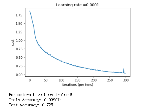
def model(X_train, Y_train, X_test, Y_test, learning_rate = 0.0001,
          num_epochs = 1500, minibatch_size = 32, print_cost = True):
    """
    Implements a three-layer tensorflow neural network: LINEAR->RELU->LINEAR->RELU->LINEAR->SOFTMAX.

    Arguments:
    X_train -- training set, of shape (input size = 12288, number of training examples = 1080)
    Y_train -- test set, of shape (output size = 6, number of training examples = 1080)
    X_test -- training set, of shape (input size = 12288, number of training examples = 120)
    Y_test -- test set, of shape (output size = 6, number of test examples = 120)
    learning_rate -- learning rate of the optimization
    num_epochs -- number of epochs of the optimization loop
    minibatch_size -- size of a minibatch
    print_cost -- True to print the cost every 100 epochs

    Returns:
    parameters -- parameters learnt by the model. They can then be used to predict.
    """

    ops.reset_default_graph()                         # to be able to rerun the model without overwriting tf variables
    tf.set_random_seed(1)                             # to keep consistent results
    seed = 3                                          # to keep consistent results
    (n_x, m) = X_train.shape                          # (n_x: input size, m : number of examples in the train set)
    n_y = Y_train.shape[0]                            # n_y : output size
    costs = []                                        # To keep track of the cost

    # Create Placeholders of shape (n_x, n_y)
    ### START CODE HERE ### (1 line)
    X, Y = create_placeholders(n_x, n_y)
    ### END CODE HERE ###

    # Initialize parameters
    ### START CODE HERE ### (1 line)
    parameters = initialize_parameters()
    ### END CODE HERE ###

    # Forward propagation: Build the forward propagation in the tensorflow graph
    ### START CODE HERE ### (1 line)
    Z3 = forward_propagation(X, parameters)
    ### END CODE HERE ###

    # Cost function: Add cost function to tensorflow graph
    ### START CODE HERE ### (1 line)
    cost = compute_cost(Z3, Y)
    ### END CODE HERE ###

    # Backpropagation: Define the tensorflow optimizer. Use an AdamOptimizer.
    ### START CODE HERE ### (1 line)
    optimizer = tf.train.AdamOptimizer(learning_rate = learning_rate).minimize(cost)
    ### END CODE HERE ###

    # Initialize all the variables
    init = tf.global_variables_initializer()

    # Start the session to compute the tensorflow graph
    with tf.Session() as sess:

        # Run the initialization
        sess.run(init)

        # Do the training loop
        for epoch in range(num_epochs):

            epoch_cost = 0.                       # Defines a cost related to an epoch
            num_minibatches = int(m / minibatch_size) # number of minibatches of size minibatch_size in the train set
            seed = seed + 1
            minibatches = random_mini_batches(X_train, Y_train, minibatch_size, seed)

            for minibatch in minibatches:

                # Select a minibatch
                (minibatch_X, minibatch_Y) = minibatch

                # IMPORTANT: The line that runs the graph on a minibatch.
                # Run the session to execute the "optimizer" and the "cost", the feedict should contain a minibatch for (X,Y).
                ### START CODE HERE ### (1 line)
                _ , minibatch_cost = sess.run([optimizer, cost], feed_dict={X: minibatch_X, Y: minibatch_Y})
                ### END CODE HERE ###

                epoch_cost += minibatch_cost / num_minibatches

            # Print the cost every epoch
            if print_cost == True and epoch % 100 == 0:
                print ("Cost after epoch %i: %f" % (epoch, epoch_cost))
            if print_cost == True and epoch % 5 == 0:
                costs.append(epoch_cost)

        # plot the cost
        plt.plot(np.squeeze(costs))
        plt.ylabel('cost')
        plt.xlabel('iterations (per tens)')
        plt.title("Learning rate =" + str(learning_rate))
        plt.show()

        # lets save the parameters in a variable
        parameters = sess.run(parameters)
        print ("Parameters have been trained!")

        # Calculate the correct predictions
        correct_prediction = tf.equal(tf.argmax(Z3), tf.argmax(Y))

        # Calculate accuracy on the test set
        accuracy = tf.reduce_mean(tf.cast(correct_prediction, "float"))

        print ("Train Accuracy:", accuracy.eval({X: X_train, Y: Y_train}))
        print ("Test Accuracy:", accuracy.eval({X: X_test, Y: Y_test}))

        return parameters
我们执行:
parameters = model(X_train, Y_train, X_test, Y_test)
得到结果:

tensorflow的 函数库很多,这里是冰山一角,还有很多需要我们去学习。后面有时间,就把图像识别的卷积的tensorflow例子给搬出研究一下。
我的大都内容来自吴恩达的公益视频和教案,特此鸣谢。
参考:吴恩达网易课程