今天是看的逻辑回归的案例。和先前一样,由于使用的TF2.0改用了网络上的代码。
同时,虽然代码成功运行,但是逻辑回归算法的原理和很多地方的“为什么这么写”仍然没有弄得很清楚。目前正在参考一篇博客(链接https://blog.csdn.net/weixin_39445556/article/details/83930186)但一时半会仍然没有弄懂。不过这个和先前的线性回归部分都明显体会到了 计算机做事本质是“让计算机解数学题”这一点。
代码如下(来源:https://blog.csdn.net/wardseptember/article/details/101910382)


 1 import tensorflow as tf
 2 import numpy as np
 3 import matplotlib.pyplot as plt
 4
 5 #import mnist in TF2.0
 6 from tensorflow.keras.datasets import mnist
 7
 8 #Disable TF2 behavior
 9 #tf.disable_v2_behavior()
10 #Disable executing eagerly
11 #tf.compat.v1.disable_eager_execution();
12 #check whether the executing eagerly is Enabled
13 tf.executing_eagerly();
14
15 #VALUE
16 #MNIST
17 num_classes = 10
18 num_features = 784
19 #train
20 learning_rate = 0.01
21 training_steps = 1000
22 batch_size = 256
23 display_step = 50
24
25 #primary Code(s) starts here
26 # 预处理数据集
27 (x_train, y_train), (x_test, y_test) = mnist.load_data()
28 # 转为float32
29 x_train, x_test = np.array(x_train, np.float32), np.array(x_test, np.float32)
30 # 转为一维向量
31 x_train, x_test = x_train.reshape([-1, num_features]), x_test.reshape([-1, num_features])
32 # [0, 255] 到 [0, 1]
33 x_train, x_test = x_train / 255, x_test / 255
34
35 # tf.data.Dataset.from_tensor_slices 是使用x_train, y_train构建数据集
36 train_data = tf.data.Dataset.from_tensor_slices((x_train, y_train))
37 # 将数据集打乱,并设置batch_size大小
38 train_data = train_data.repeat().shuffle(5000).batch(batch_size).prefetch(1)
39
40 # 权重[748, 10],图片大小28*28,类数
41 W = tf.Variable(tf.ones([num_features, num_classes]), name="weight")
42 # 偏置[10],共10类
43 b = tf.Variable(tf.zeros([num_classes]), name="bias")
44
45 # 逻辑回归函数
46 def logistic_regression(x):
47     return tf.nn.softmax(tf.matmul(x, W) + b)
48
49 # 损失函数
50 def cross_entropy(y_pred, y_true):
51     # tf.one_hot()函数的作用是将一个值化为一个概率分布的向量
52     y_true = tf.one_hot(y_true, depth=num_classes)
53     # tf.clip_by_value将y_pred的值控制在1e-9和1.0之间
54     y_pred = tf.clip_by_value(y_pred, 1e-9, 1.0)
55     return tf.reduce_mean(-tf.reduce_sum(y_true * tf.math.log(y_pred)))
56
57 # 计算精度
58 def accuracy(y_pred, y_true):
59     # tf.cast作用是类型转换
60     correct_prediction = tf.equal(tf.argmax(y_pred, 1), tf.cast(y_true, tf.int64))
61     return tf.reduce_mean(tf.cast(correct_prediction, tf.float32))
62
63 # 优化器采用随机梯度下降
64 optimizer = tf.optimizers.SGD(learning_rate)
65
66 # 梯度下降
67 def run_optimization(x, y):
68     with tf.GradientTape() as g:
69         pred = logistic_regression(x)
70         loss = cross_entropy(pred, y)
71     # 计算梯度
72     gradients = g.gradient(loss, [W, b])
73     # 更新梯度
74     optimizer.apply_gradients(zip(gradients, [W, b]))
75
76 # 开始训练
77 for step, (batch_x, batch_y) in enumerate(train_data.take(training_steps), 1):
78     run_optimization(batch_x, batch_y)
79     if step % display_step == 0:
80         pred = logistic_regression(batch_x)
81         loss = cross_entropy(pred, batch_y)
82         acc = accuracy(pred, batch_y)
83         print("step: %i, loss: %f, accuracy: %f" % (step, loss, acc))
84
85 # 测试模型的准确率
86 pred = logistic_regression(x_test)
87 print("Test Accuracy: %f" % accuracy(pred, y_test))
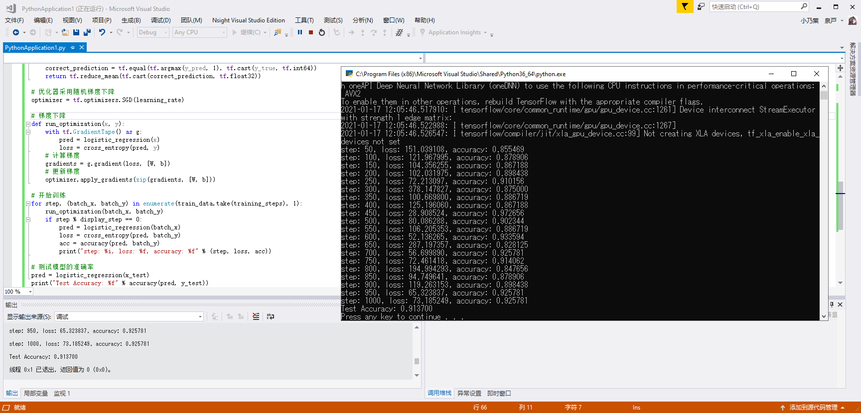
运行结果如下: