20210115

今天是写一个线性回归的实例。

但是由于TF1.X和TF2.X的区别，所给的教学视频里的实例已完全不可用(除非禁用掉全部TF2.0特性)，因而转为自行找到了一个实例修改为视讯里的参数后运行。不过所给实例里的两个参数并未给出，个人只能指定一个猜测的数值。

代码如下（来源：https://blog.csdn.net/weixin_43584807/article/details/105784040）

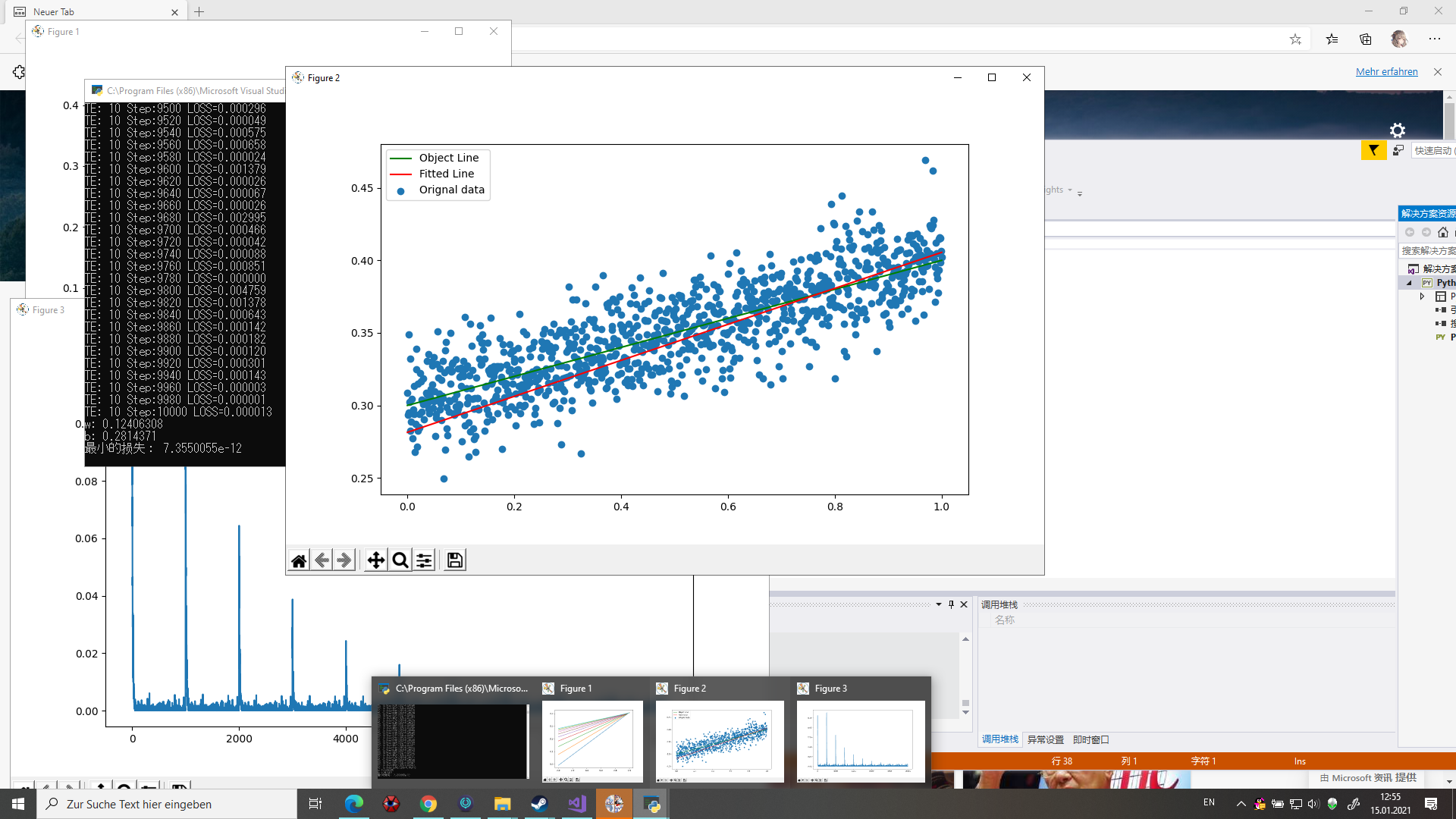
 1 import tensorflow as tf
 2 import numpy as np
 3 import matplotlib.pyplot as plt
 4 
 5 #Disable TF2 behavior
 6 #tf.disable_v2_behavior()
 7 #Disable executing eagerly
 8 #tf.compat.v1.disable_eager_execution();
 9 #check whether the executing eagerly is Enabled
10 tf.executing_eagerly();
11 
12 #VALUE
13 training_epochs = 10
14 learning_rate = 0.02
15 
16 #primary Code(s) starts here
17 num_points = 1000
18 def data():
19     x_data = np.linspace(0,1,1000)
20     np.random.seed(5)
21     ## y=3.1234*x+2.98+噪声（噪声的维度要和x_data一致）
22     y_data = 0.1 * x_data + 0.3 + np.random.randn(*x_data.shape) * 0.02
23     return x_data,y_data
24 
25 x_data,y_data = data()
26 
27 w = tf.Variable(np.random.randn(),tf.float32)
28 ##构建模型中的变量b，对应线性函数的截距
29 b = tf.Variable(0.0,tf.float32)
30 def y_function(x,w,b):
31     return w * x + b
32 def loss(x,y,w,b):
33     return tf.reduce_mean(tf.square(y_function(x,w,b)-y))
34 def grad(x,y,w,b):
35     with tf.GradientTape() as tape:
36         loss_ = loss(x,y,w,b)
37     return tape.gradient(loss_,[w,b])
38 
39 step = 0
40 loss_list = [] #List of loss value
41 display_step = 10
42 for epoch in range(training_epochs):
43     for xs,ys in zip(x_data,y_data):
44         loss_ = loss(xs,ys,w,b)
45         loss_list.append(loss_)
46         delta_w,delta_b = grad(xs,ys,w,b)
47         change_w = delta_w * learning_rate
48         change_b = delta_b * learning_rate
49         w.assign_sub(change_w)
50         b.assign_sub(change_b)
51         step=step+1;
52         if step%(2*display_step)==0:
53             print("TE:",'%02d'%(epoch+1),"Step:%03d"%(step),"LOSS=%.6f"%(loss_))
54     plt.plot(x_data,w.numpy()*x_data+b.numpy())
55 print('w:',w.numpy())
56 print('b:',b.numpy())
57 print('最小的损失：',min(loss_list).numpy())
58 plt.figure(figsize=(10,6))
59 plt.scatter(x_data,y_data,label='Orignal data')
60 plt.plot(x_data, 0.1 * x_data + 0.3, label ='Object Line',c='g')
61 plt.plot(x_data, x_data * w.numpy() + b.numpy(), label='Fitted Line',color='r')
62 plt.legend(loc=2)
63 plt.figure(figsize=(10,6))
64 plt.plot(loss_list)
65 plt.show()

View Code

运行结果：