PR曲线、LDA、决策树实例分析

1. 请阐述监督学习，半监督学习，无监督学习和弱监督学习区别

• 监督学习：
  给定数据，预测标签。通过已有的一部分输入数据与输出数据之间的对应关系，生成一个函数，将输入映射到合适的输出，例如分类。
• 半监督学习：
  但是使用的数据，一部分是标记过的，而大部分是没有标记的。综合利用有类标的和没有类标的数据，来生成合适的分类函数。和监督学习相比较，半监督学习的成本较低，但是又能达到较高的准确度。
• 无监督学习：
  只有特征，没有标签。给定输入数据，寻找隐藏的关系。如在只有特征，没有标签的训练数据集中，通过数据之间的内在联系和相似性将他们分成若干类。
• 弱监督学习：
  弱监督学习主要可以分为三类：不完全监督，即只有一部分样本有标签；不确切监督，即训练样本只有粗粒度的标签；不准确监督，即给定的标签不一定总是真值。

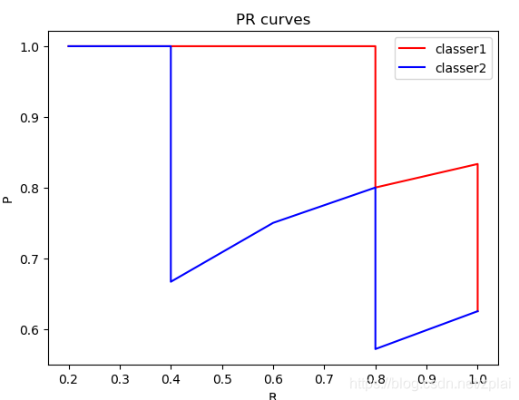
2. 请画出以下两个分类器分类 PR 曲线

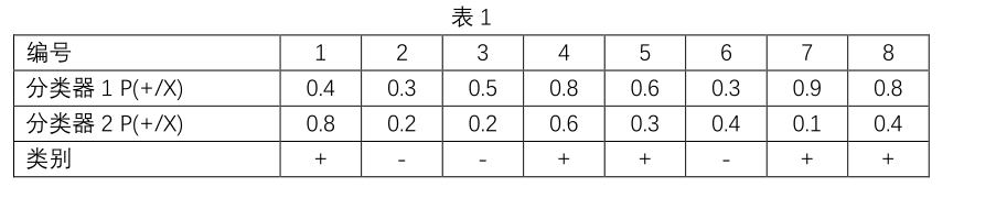
• 对分类器1按(P(+/X))从大到小排序：

	+	+	+	+	-	+	-	-
P	1/1	2/2	3/3	4/4	4/5	5/6	5/7	5/8
R	1/5	2/5	3/5	4/5	4/5	5/5	5/5	5/5

• 对分类器2按(P(+/X))从大到小排序(r若相等则按原顺序)：

	+	+	-	+	+	-	-	+
P	1/1	2/2	2/3	3/4	4/5	4/6	4/7	5/8
R	1/5	2/5	2/5	3/5	4/5	4/5	4/5	5/5

PR曲线如下：

代码如下：

from fractions import Fraction
from matplotlib import pyplot as plt

tag = ['+', '-', '-', '+', '+', '-', '+', '+']
array1 = [0.4, 0.3, 0.5, 0.8, 0.6, 0.3, 0.9, 0.8]
array2 = [0.8, 0.2, 0.2, 0.6, 0.3, 0.4, 0.1, 0.4]
classer1 = list(zip(tag, array1))
classer2 = list(zip(tag, array2))
classer1.sort(key = lambda x: -x[1])
classer2.sort(key = lambda x: -x[1])
print(classer1)
print(classer2)
total_1 = tag.count('+')
p1 = []
r1 = []
now_1 = 0
for i, item in enumerate(classer1):
	if item[0] == '+':
		now_1 += 1
	p1.append(now_1 / (i+1))
	r1.append(now_1 / total_1)

p2 = []
r2 = []
now_1 = 0
for i, item in enumerate(classer2):
	if item[0] == '+':
		now_1 += 1
	p2.append(now_1 / (i+1))
	r2.append(now_1 / total_1)


plt.title('PR curves')
plt.xlabel('R')
plt.ylabel('P')
plt.plot(r1, p1, color = 'r', label = 'classer1')
plt.plot(r2, p2, color = 'b', label = 'classer2')
plt.legend()
plt.show()

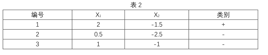
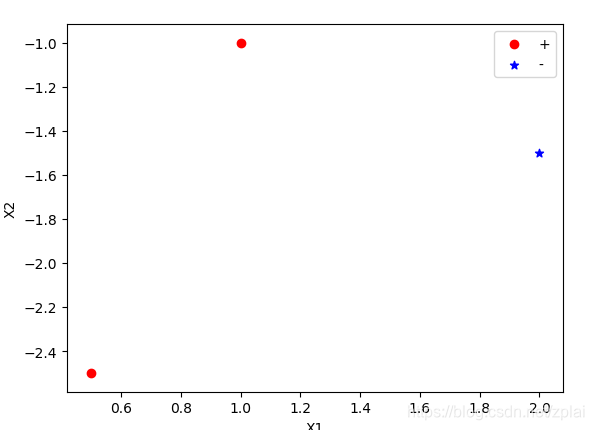
3. 请用表 2 中数据集，计算 LDA 最大化目标

[egin{gathered} X = quad egin{bmatrix} 2 & 0.5 & 1\ -1.5 & -2.5 & -1 end{bmatrix} quad X0 = quad egin{bmatrix} 0.5 & 1 \ -2.5 &-1 end{bmatrix} quad X1 = quad egin{bmatrix} 2 \ -1.5 end{bmatrix} quad end{gathered} ]

[u0 = quad egin{bmatrix} 0.75 \ -1.75 end{bmatrix} quad u1 = quad egin{bmatrix} 2 \ -1.5 end{bmatrix} quad ]

[S_w = sum_{0} + sum_{1} ]

[S_w = sum_{xin X0}(x-u0)(x-u0)^T+ sum_{xin X1}(x-u1)(x-u1)^T ]

[egin{gathered} S_w = quad egin{bmatrix} -0.25 \ -0.75 end{bmatrix} quad quad egin{bmatrix} -0.25 & -0.75 end{bmatrix} quad + quad egin{bmatrix} 0.25 \ 0.75 end{bmatrix} quad quad egin{bmatrix} 0.25 & 0.75 end{bmatrix} quad +0 = quad egin{bmatrix} frac{1}{8} & frac{3}{8} \ frac{3}{8} & frac{9}{8} end{bmatrix} quad end{gathered} ]

[S_b =(u0-u1)(u0-u1)^T ]

[egin{gathered} S_b = quad egin{bmatrix} -1.25 \ -0.25 end{bmatrix} quad quad egin{bmatrix} -1.25 & -0.25 end{bmatrix} quad = quad egin{bmatrix} frac{25}{16} & frac{5}{16} \ frac{5}{16} & frac{1}{16} end{bmatrix} quad end{gathered} ]

[egin{gathered} w = S_w^{-1}(u0-u1)= quad egin{bmatrix} -0.16 \ -0.48 end{bmatrix} quad end{gathered} ]

[J = frac{W^TS_bW}{W^TS_wW} = 0.32 ]

代码：

import numpy as np
from matplotlib import pyplot as plt

x = np.array([[2, 0.5, 1],[-1.5, -2.5, -1]])
y = np.array([1, 0, 0]).reshape(1, 3)
tag0 = y.repeat(repeats = x.shape[0], axis = 0) == 0
x0 = x[tag0].reshape(tag0.shape[0], np.sum(tag0[0]))
tag1 = y.repeat(repeats = x.shape[0], axis = 0) == 1
x1 = x[tag1].reshape(tag1.shape[0], np.sum(tag1[0]))
u0 = np.mean(x0, axis = 1).reshape(x0.shape[0], 1)
u1 = np.mean(x1, axis = 1).reshape(x0.shape[0], 1)
sigma0 = np.zeros((x0.shape[0], x0.shape[0]))
# print(x0, '
', x1, '
', u0, '
', u1, '
', sigma0)
for i in np.arange(x0.shape[1]):
	x_t = x0[:, i].reshape(x0.shape[0], 1) - u0
	print(x_t)
	sigma0 += np.dot(x_t, x_t.T) 
print(sigma0)

sigma1 = np.zeros((x1.shape[0], x1.shape[0]))
for i in np.arange(x1.shape[1]):
	x_t = x1[:, i].reshape(x1.shape[0], 1) - u1
	print(x_t)
	sigma1 += np.dot(x_t, x_t.T)
print(sigma1)

sw = sigma0 + sigma1
sw_inv = np.linalg.pinv(sw)
sb = np.dot(u0-u1, (u0-u1).T)

w = sw_inv.dot(u0-u1)
j = w.T.dot(sb).dot(w) / w.T.dot(sw).dot(w)
print(w, '
', sw, '
', sb, '
', j)
print(w.T.dot(x))

plt.xlabel('X1')
plt.ylabel('X2')
x01 = x0[0, :]
x02 = x0[1, :]
plt.scatter(x01, x02, color = 'r', marker = 'o', label = '+')
#plt.plot(x01, x02, 'or')
x11 = x1[0, :]
x12 = x1[1, :]
plt.scatter(x11, x12, color = 'b', marker = '*', label = '-')
# plt.plot(x11, x12, '+b')
plt.legend()
plt.show()

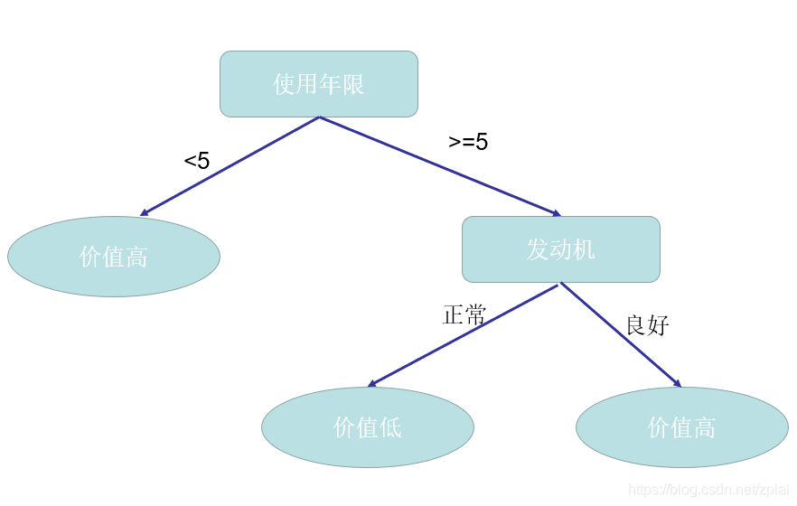
4. 请用表 3 中数据集，利用信息增益生成决策树，并写出计算过程。假设属性使用年限阈值设置为 5。

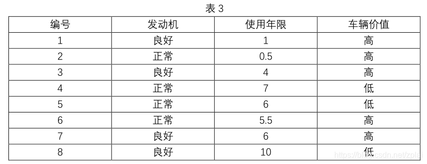
(Ent(D)=-frac{5}{8}log_2frac{5}{8}--frac{3}{8}log_2frac{3}{8}=0.9544)
若按发动机状态划分：
(Ent(D^{良好})=-frac{3}{4}log_2frac{3}{4}--frac{1}{4}log_2frac{1}{4}=0.8113)
(Ent(D^{正常})=-frac{2}{4}log_2frac{2}{4}--frac{2}{4}log_2frac{2}{4}=1)
(Gain(D, 发动机) = Ent(D) - Ent(D^{良好})- Ent(D^{正常}) = 0.0488)
若按使用年限划分：
(Ent(D^{geq5})=-frac{3}{3}log_{2}frac{3}{3}--0log_{2}0=0)
(Ent(D^{ geq5})=-frac{3}{5}log_{2}frac{3}{5}--frac{2}{5}log_{2}frac{2}{5}=0.9710)
(Gain(D, 使用年限) = Ent(D) - Ent(D^{geq5})- Ent(D^{ geq5}) = 0.3475)
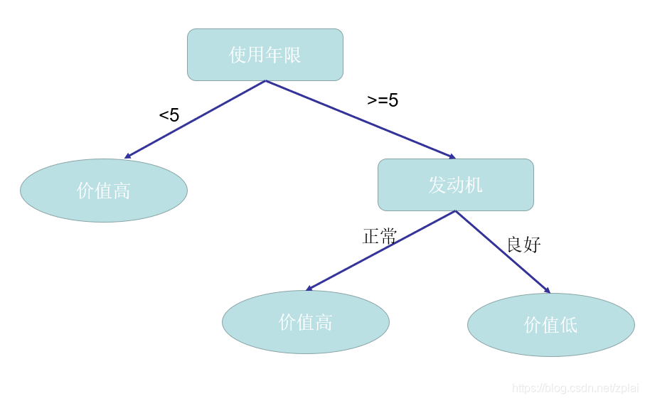
(Gain(D,使用年限)>Gain(D,发动机))
则首先按使用年限作为划分结点，可得如下决策树：

或