注意力机制及Keras实现

注意力往往与encoder-decoder（seq2seq）框架搭在一起，假设我们编码前与解码后的序列如下：

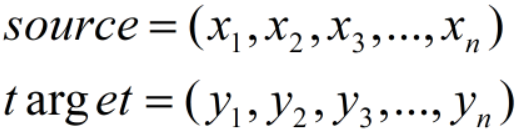
 编码时，我们将source通过非线性变换到中间语义：

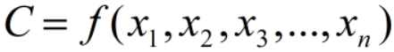
 则我们解码时，第i个输出为：

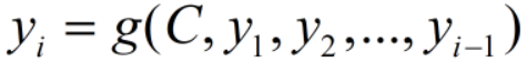
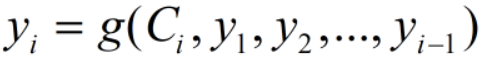
 可以看到，不管i为多少，都是基于相同的中间语义C进行解码的，也就是说，我们的注意力对所有输出都是相同的。所以，注意力机制的任务就是突出重点，也就是说，我们的中间语义C对不同i应该有不同的侧重点，即上式变为：

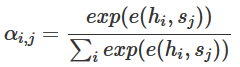
常见的有Bahdanau Attention

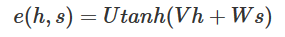
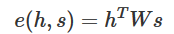
 e(h,s)代表一层全连接层。

及Luong Attention

---

学习的一个github上的代码，分析了一下实现过程。代码下载链接：https://github.com/Choco31415/Attention_Network_With_Keras

代码的主要目标是通过一个描述时间的字符串，预测为数字形式的字符串。如“ten before ten o'clock a.m”预测为09:50

在jupyter上运行，代码如下：

1，导入模块，好像并没有全部使用到，如Permute，Multiply，Reshape，LearningRateScheduler等

from keras.layers import Bidirectional, Concatenate, Permute, Dot, Input, LSTM, Multiply, Reshape
from keras.layers import RepeatVector, Dense, Activation, Lambda
from keras.optimizers import Adam
#from keras.utils import to_categorical
from keras.models import load_model, Model
#from keras.callbacks import LearningRateScheduler
import keras.backend as K

import matplotlib.pyplot as plt
%matplotlib inline

import random
#import math

import json
import numpy as np

 2，加载数据集，以及翻译前和翻译后的词典

with open('data/Time Dataset.json','r') as f:
    dataset = json.loads(f.read())
with open('data/Time Vocabs.json','r') as f:
    human_vocab, machine_vocab = json.loads(f.read())
    
human_vocab_size = len(human_vocab)
machine_vocab_size = len(machine_vocab)

这里human_vocab词典是将每个字符映射到索引，machine_vocab是将翻译后的字符映射到索引，因为翻译后的时间只包含0-9以及冒号：

3，定义数据处理方法

def preprocess_data(dataset, human_vocab, machine_vocab, Tx, Ty):
    """
    A method for tokenizing data.
    
    Inputs:
    dataset - A list of sentence data pairs.
    human_vocab - A dictionary of tokens (char) to id's.
    machine_vocab - A dictionary of tokens (char) to id's.
    Tx - X data size
    Ty - Y data size
    
    Outputs:
    X - Sparse tokens for X data
    Y - Sparse tokens for Y data
    Xoh - One hot tokens for X data
    Yoh - One hot tokens for Y data
    """
    
    # Metadata
    m = len(dataset)
    
    # Initialize
    X = np.zeros([m, Tx], dtype='int32')
    Y = np.zeros([m, Ty], dtype='int32')
    
    # Process data
    for i in range(m):
        data = dataset[i]
        X[i] = np.array(tokenize(data[0], human_vocab, Tx))
        Y[i] = np.array(tokenize(data[1], machine_vocab, Ty))
    
    # Expand one hots
    Xoh = oh_2d(X, len(human_vocab))
    Yoh = oh_2d(Y, len(machine_vocab))
    
    return (X, Y, Xoh, Yoh)
    
def tokenize(sentence, vocab, length):
    """
    Returns a series of id's for a given input token sequence.
    
    It is advised that the vocab supports <pad> and <unk>.
    
    Inputs:
    sentence - Series of tokens
    vocab - A dictionary from token to id
    length - Max number of tokens to consider
    
    Outputs:
    tokens - 
    """
    tokens = [0]*length
    for i in range(length):
        char = sentence[i] if i < len(sentence) else "<pad>"
        char = char if (char in vocab) else "<unk>"
        tokens[i] = vocab[char]
        
    return tokens

def ids_to_keys(sentence, vocab):
    """
    Converts a series of id's into the keys of a dictionary.
    """
    reverse_vocab = {v: k for k, v in vocab.items()}
    
    return [reverse_vocab[id] for id in sentence]

def oh_2d(dense, max_value):
    """
    Create a one hot array for the 2D input dense array.
    """
    # Initialize
    oh = np.zeros(np.append(dense.shape, [max_value]))
#     oh=np.zeros((dense.shape[0],dense.shape[1],max_value)) 这样写更为直观
    
    # Set correct indices
    ids1, ids2 = np.meshgrid(np.arange(dense.shape[0]), np.arange(dense.shape[1]))
    
#     'F'表示一列列的展开，默认按行展开。将id序列中每个数字再one-hot化。
    oh[ids1.flatten(), ids2.flatten(), dense.flatten('F').astype(int)] = 1
    
    return oh

4，输入中最长的字符串为41，输出长度都是5，训练测试数据使用one-hot编码后的，训练集占比80%

Tx = 41 # Max x sequence length
Ty = 5 # y sequence length
X, Y, Xoh, Yoh = preprocess_data(dataset, human_vocab, machine_vocab, Tx, Ty)

# Split data 80-20 between training and test
train_size = int(0.8*len(dataset))
Xoh_train = Xoh[:train_size]
Yoh_train = Yoh[:train_size]
Xoh_test = Xoh[train_size:]
Yoh_test = Yoh[train_size:]

5，定义每次新预测时注意力的更新

在预测输出y_i-1后，预测y_i时，我们需要不同的注意力分布，即重新生成这个分布

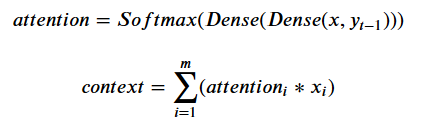
 1 # Define part of the attention layer gloablly so as to
 2 # share the same layers for each attention step.
 3 def softmax(x):
 4     return K.softmax(x, axis=1)
 5 # 重复矢量，用于将一个矢量扩展成一个维度合适的tensor
 6 at_repeat = RepeatVector(Tx)
 7 # 在最后一位进行维度合并
 8 at_concatenate = Concatenate(axis=-1)
 9 at_dense1 = Dense(8, activation="tanh")
10 at_dense2 = Dense(1, activation="relu")
11 at_softmax = Activation(softmax, name='attention_weights')
12 # 这里参数名为axes。。虽然和axis是一个意思
13 at_dot = Dot(axes=1)
14 
15 # 每次新的预测的时候都需要更新attention
16 def one_step_of_attention(h_prev, a):
17     """
18     Get the context.
19     
20     Input:
21     h_prev - Previous hidden state of a RNN layer (m, n_h)
22     a - Input data, possibly processed (m, Tx, n_a)
23     
24     Output:
25     context - Current context (m, Tx, n_a)
26     """
27     # Repeat vector to match a's dimensions
28     h_repeat = at_repeat(h_prev)
29     # Calculate attention weights
30     i = at_concatenate([a, h_repeat]) #对应公式中x和yt-1合并
31     i = at_dense1(i)#对应公式中第一个Dense
32     i = at_dense2(i)#第二个Dense
33     attention = at_softmax(i)#Softmax，此时得到一个注意力分布
34     # Calculate the context
35 #     这里使用新的attention与输入相乘，即注意力的核心原理：对于输入产生某种偏好分布
36     context = at_dot([attention, a])#Dot，使用注意力偏好分布作用于输入，返回更新后的输入
37     
38     return context

以上，注意力的计算公式如下所示：

 6，定义注意力层

def attention_layer(X, n_h, Ty):
    """
    Creates an attention layer.
    
    Input:
    X - Layer input (m, Tx, x_vocab_size)
    n_h - Size of LSTM hidden layer
    Ty - Timesteps in output sequence
    
    Output:
    output - The output of the attention layer (m, Tx, n_h)
    """    
    # Define the default state for the LSTM layer
#     Lambda层不需要训练参数，这里初始化状态
    h = Lambda(lambda X: K.zeros(shape=(K.shape(X)[0], n_h)))(X)
    c = Lambda(lambda X: K.zeros(shape=(K.shape(X)[0], n_h)))(X)
    # Messy, but the alternative is using more Input()
    
    at_LSTM = LSTM(n_h, return_state=True)
    
    output = []
              
    # Run attention step and RNN for each output time step
　　　　# 这里就是每次预测时，先更新context，用这个新的context通过LSTM获得各个输出h
    for _ in range(Ty):
#         第一次使用初始化的注意力参数作用输入X，之后使用上一次的h作用输入X，保证每次预测的时候注意力都对输入产生偏好
        context = one_step_of_attention(h, X)
#         得到新的输出
        h, _, c = at_LSTM(context, initial_state=[h, c])
        
        output.append(h)
#     返回全部输出
    return output

7，定义模型

 1 layer3 = Dense(machine_vocab_size, activation=softmax)
 2 layer1_size=32
 3 layer2_size=64
 4 def get_model(Tx, Ty, layer1_size, layer2_size, x_vocab_size, y_vocab_size):
 5     """
 6     Creates a model.
 7     
 8     input:
 9     Tx - Number of x timesteps
10     Ty - Number of y timesteps
11     size_layer1 - Number of neurons in BiLSTM
12     size_layer2 - Number of neurons in attention LSTM hidden layer
13     x_vocab_size - Number of possible token types for x
14     y_vocab_size - Number of possible token types for y
15     
16     Output:
17     model - A Keras Model.
18     """
19     
20     # Create layers one by one
21     X = Input(shape=(Tx, x_vocab_size))
22     # 使用双向LSTM
23     a1 = Bidirectional(LSTM(layer1_size, return_sequences=True), merge_mode='concat')(X)
24     
25 #     注意力层
26     a2 = attention_layer(a1, layer2_size, Ty)
27     # 对输出h应用一个Dense得到最后输出y
28     a3 = [layer3(timestep) for timestep in a2]
29         
30     # Create Keras model
31     model = Model(inputs=[X], outputs=a3)
32     
33     return model

8，训练模型

model = get_model(Tx, Ty, layer1_size, layer2_size, human_vocab_size, machine_vocab_size)
#这里我们可以看下模型的构成，需要提前安装graphviz模块
from keras.utils import plot_model
#在当前路径下生成模型各层的结构图，自己去看看理解
plot_model(model,show_shapes=True,show_layer_names=True)
opt = Adam(lr=0.05, decay=0.04, clipnorm=1.0)
model.compile(optimizer=opt, loss='categorical_crossentropy', metrics=['accuracy'])
# (8000,5,11)->(5,8000,11)，以时间序列而非样本序列去训练，因为多个样本间是没有“序”的关系的，这样RNN也学不到啥东西
outputs_train = list(Yoh_train.swapaxes(0,1))
model.fit([Xoh_train], outputs_train, epochs=30, batch_size=100,verbose=2

如下为模型的结构图

9，评估

outputs_test = list(Yoh_test.swapaxes(0,1))
score = model.evaluate(Xoh_test, outputs_test) 
print('Test loss: ', score[0])

10，预测

这里就随机对数据集中的一个样本进行预测

i = random.randint(0, len(dataset))

def get_prediction(model, x):
    prediction = model.predict(x)
    max_prediction = [y.argmax() for y in prediction]
    str_prediction = "".join(ids_to_keys(max_prediction, machine_vocab))
    return (max_prediction, str_prediction)

max_prediction, str_prediction = get_prediction(model, Xoh[i:i+1])

print("Input: " + str(dataset[i][0]))
print("Tokenized: " + str(X[i]))
print("Prediction: " + str(max_prediction))
print("Prediction text: " + str(str_prediction))

11，还可以查看一下注意力的图像

i = random.randint(0, len(dataset))

def plot_attention_graph(model, x, Tx, Ty, human_vocab, layer=7):
    # Process input
    tokens = np.array([tokenize(x, human_vocab, Tx)])
    tokens_oh = oh_2d(tokens, len(human_vocab))
    
    # Monitor model layer
    layer = model.layers[layer]
    
    layer_over_time = K.function(model.inputs, [layer.get_output_at(t) for t in range(Ty)])
    layer_output = layer_over_time([tokens_oh])
    layer_output = [row.flatten().tolist() for row in layer_output]
    
    # Get model output
    prediction = get_prediction(model, tokens_oh)[1]
    
    # Graph the data
    fig = plt.figure()
    fig.set_figwidth(20)
    fig.set_figheight(1.8)
    ax = fig.add_subplot(111)
    
    plt.title("Attention Values per Timestep")
    
    plt.rc('figure')
    cax = plt.imshow(layer_output, vmin=0, vmax=1)
    fig.colorbar(cax)
    
    plt.xlabel("Input")
    ax.set_xticks(range(Tx))
    ax.set_xticklabels(x)
    
    plt.ylabel("Output")
    ax.set_yticks(range(Ty))
    ax.set_yticklabels(prediction)
    
    plt.show()
# 这个图像如何看：先看纵坐标，从上到下，为15:48，生成1和5时注意力在four这个单词上，生成48分钟的时候注意力集中在before单词上，这个例子非常好
plot_attention_graph(model, dataset[i][0], Tx, Ty, human_vocab)

如图所示，在预测1和5时注意力在four单词上，预测4，8时注意力在before单词上，这比较符合逻辑。