Numpy


numpy数据类型

1.为啥使用numpy ?
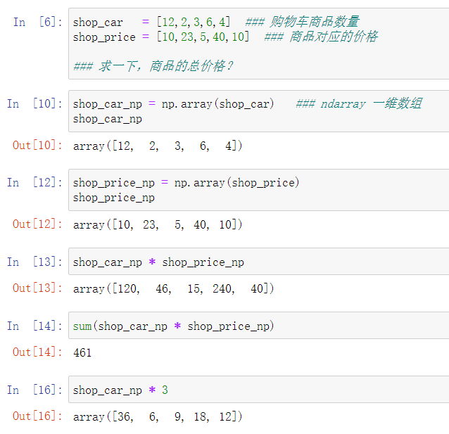
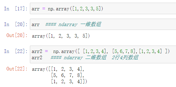
ndarray是一个多维数组列表
Numpy的核心特征就是N-维数组对----ndarray
它和python中的列表区别:
1.数组对象内元素类型必须相同
2.数组大小不可修改
2.创建ndarray 数组
# 创建方法
# np.array(array_like)   # array_like可以是列表,可迭代对象等像数据的数据
listnp = np.array([1,2,3,4,5,6])
rangenp = np.array(range(10))
把一维数组转换成三维数组
a = np.arange(15)
# print(a)
print(a.shape)  # (15,)
b = a.reshape((3,5))
'''
[[ 0  1  2  3  4]
 [ 5  6  7  8  9]
 [10 11 12 13 14]]
'''
print(b)
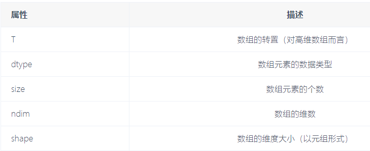
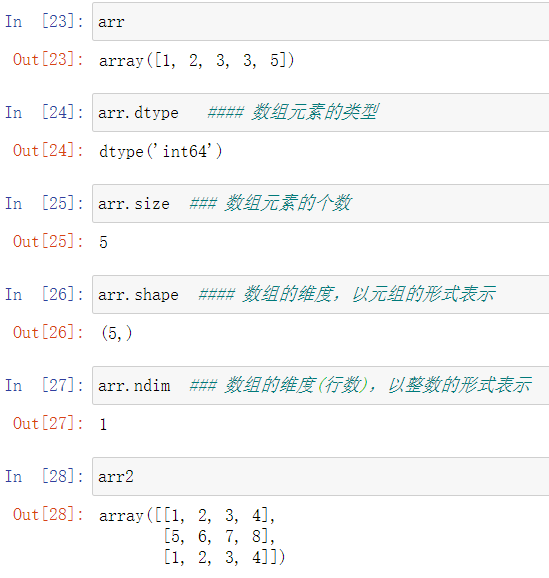
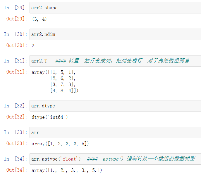
3.常见的属性
数据类型

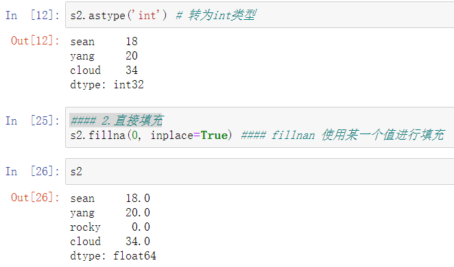
astype()方法可以修改数组类型
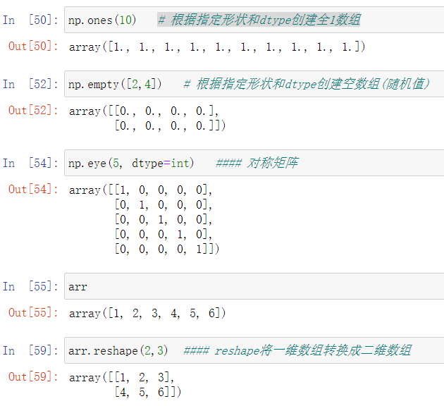
4.ndarray的创建方式
注:empty创建,使用未使用的物理地址。内部有值是上一次程序使用了,但是没有擦掉。这方法创建的好处是快一步,没有赋值,之后自己在赋新的值


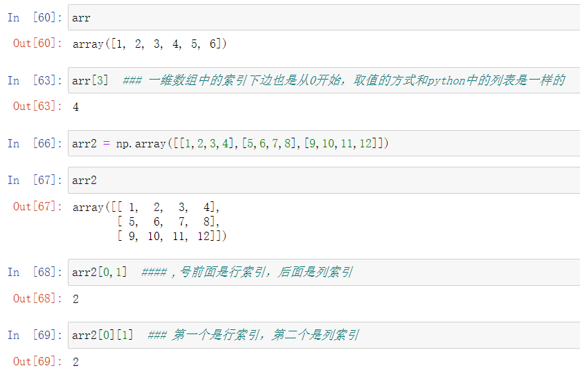
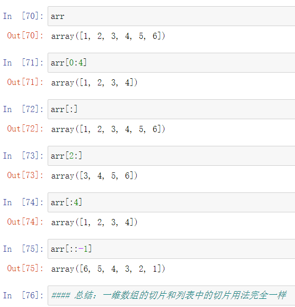
5.索引
6.切片

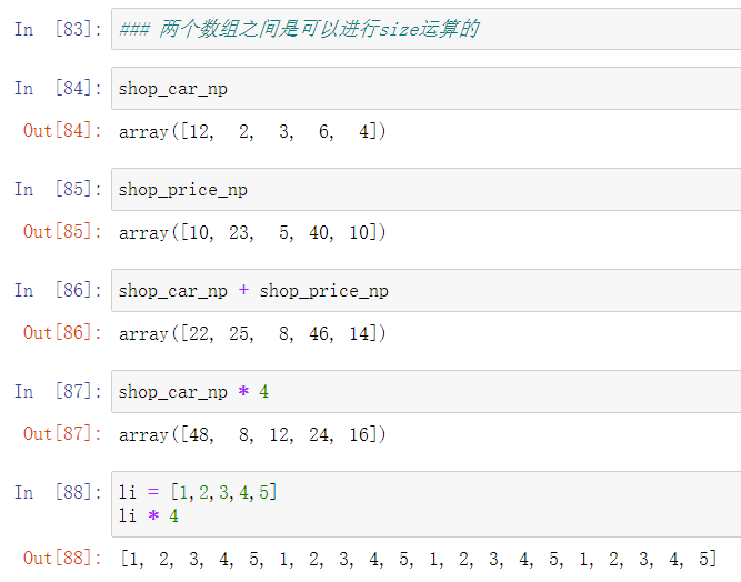
7.数组的向量运算和矢量运算
8. 布尔型索引

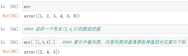
9.花式索引
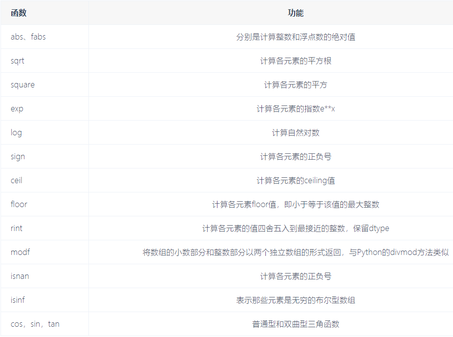
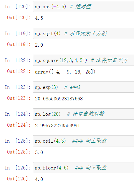
10.一元函数


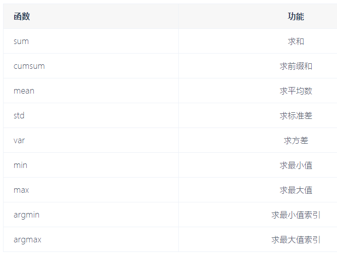
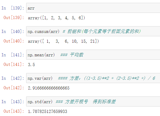
11.数学统计函数
12.随机数生成
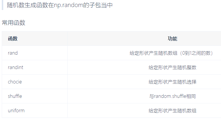

# 随机产生三维数组
a = np.random.randint(0,10,(3,5))
print(a)
'''
[[5 3 9 1 9]
 [5 1 9 6 5]
 [9 0 8 9 6]]
'''
Pandas
主要是两大数据类型, DataFrame,Series


1.Series
1.Series的创建
# 创建示例
import pandas as pd
print(pd.Series([2,3,4,5]))     # 通过列表创建
print(pd.Series(np.arange(5)))    # 通过数组创建
print(pd.Series(range(5)))  # 通过可迭代对象创建

series数据对齐
两个series数据运算处理,默认是以标签处理
# series数据对齐
sr1 = pd.Series([12,23,34],index=['c','a','d'])
sr2 = pd.Series([11,20,10],index=['d','c','a'])
print(sr1 + sr2)    # a标签相加,b标签相加,c标签相加
'''
a    33
c    32
d    45
dtype: int64
'''

# 相加缺失值
sr3 = pd.Series([12,23,34],index=['c','a','d'])
sr4 = pd.Series([11,20,10],index=['b','c','a'])
print(sr3 + sr4)
'''
a    33.0
b     NaN
c    32.0
d     NaN
dtype: float64
'''
2.缺失值处理
# 使用算术方法,add,sub,div,mul。让没有的一方赋一个值
sr1 = pd.Series([12,23,34],index=['c','a','d'])
sr2 = pd.Series([11,20,10],index=['b','c','a'])
print(sr1.add(sr2,fill_value=0))    # fill_value=0缺失部分填补为0
'''
a    33.0
b    11.0
c    32.0
d    34.0
dtype: float64
'''


sr1 = pd.Series([12,23,34],index=['c','a','d'])
sr2 = pd.Series([11,0,10],index=['b','c','a'])
# print(sr1.add(sr2,fill_value=0))    # fill_value=0缺失部分填补为0
sr = sr1/sr2
print(sr)
'''
a    2.3
b    NaN
c    inf
d    NaN
dtype: float64
'''
print(sr.isnull())  # 判断是否是缺失值NaN
'''
a    False
b     True
c    False
d     True
dtype: bool
'''
print(sr.notnull()) # 判断是否不是缺失值NaN
'''
a     True
b    False
c     True
d    False
dtype: bool
'''
print(sr[sr.notnull()]) # 过滤所有缺失值NaN
'''
a    2.3
c    inf
dtype: float64
'''
print(sr.fillna(0)) # 把缺失值NaN赋值为0
'''
a    2.3
b    0.0
c    inf
d    0.0
dtype: float64
'''
sr = sr.fillna(sr.mean()) # 把缺失值NaN赋值为sr的平均值,如果是缺失值就跳过
print(sr)   # 此处因为有inf无穷大,所以平均为无穷大
'''
a    2.3
b    inf
c    inf
d    inf
dtype: float64
'''
Series特性

注意:打印series时,是打印value,不是key
import pandas as pd
sr = pd.Series({'a':1,'b':2})
print(sr)
'''
a    1
b    2
dtype: int64
'''
for i in sr:    # 打印的是value,而不是key
    print(i)
'''
1
2
'''
in运算
import pandas as pd
sr = pd.Series({'a':1,'b':2})
print('a' in sr)    # True
print('c' in sr)    # False
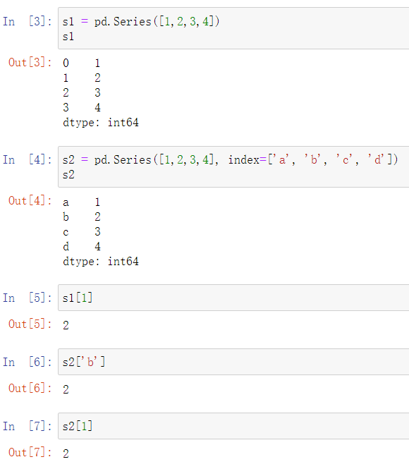
索引
注意如果是整数索引,且标签也为整数时。如s2[1],1一定会被解释为标签,而非下标!
s2 = pd.Series([1,2,3,4],index=[1,2,3,4])
print(s2)
'''
1    1
2    2
3    3
4    4
dtype: int64
'''
# print(s2[0]) # 报错
print(s2[1])    # 1 识别为标签
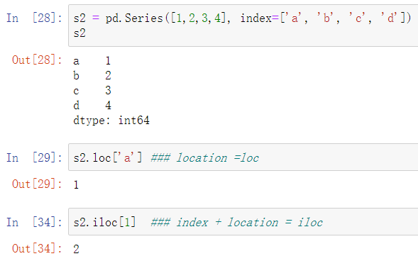
解决该方法,loc解释为标签。iloc解释为下标。
s2 = pd.Series([1,2,3,4],index=['a','b','c','d'])
print(s2)
'''
a    1
b    2
c    3
d    4
dtype: int64
'''
# location = loc
print(s2.loc['a'])  # 1
# index + location = iloc   只能写真实数字索引
print(s2.iloc[1])   # 2
# 下方写法此处解释为标签,当标签下标同时存在1时,会解释为标签1!
print(s2[1])    # 2
print(s2.iloc[0:3]) # 以下标作为索引切片
'''
a    1
b    2
c    3
dtype: int64
'''
print(s2.loc['a':'b'])  # 以标签作为索引切片
'''
a    1
b    2
dtype: int64
'''
# 花式索引
sr = pd.Series([1,2,3,4],index=['a','b','c','d'])
print(sr)
'''
a    1
b    2
c    3
d    4
dtype: int64
'''
print(sr[['a','c']])    # 花式索引,等同于sr[[0,2]]
'''
a    1
c    3
dtype: int64
'''

# 切片
print(sr['a':'c'])  # 注意如果是以标签为索引切片,前包后包
'''
a    1
b    2
c    3
dtype: int64
'''
print(sr[0:2])  # 以下标切片,前包后不包
'''
a    1
b    2
dtype: int64
'''
# 获取索引和值
import pandas as pd
sr = pd.Series({'a':1,'b':2})
print(sr)
'''
a    1
b    2
dtype: int64
'''
# 获取索引
print(sr.index) # Index(['a', 'b'], dtype='object')
print(sr.index[0])  # a
# 获取值
print(sr.values)    # [1 2]
DataFrame

# 第一种创建方式
df1 = pd.DataFrame({'one':[1,2,3],'two':[4,5,6]},index=['a','b','c'])
print(df1)
'''
   one  two
a    1    4
b    2    5
c    3    6
'''
# 第二种创建方式
df2 = pd.DataFrame({'one':pd.Series([1,2,3],index=['a','b','c']),'two':pd.Series([1,2,3,4],index=['b','a','c','d'])})
print(df2)
'''
   one  two
a  1.0    2
b  2.0    1
c  3.0    3
d  NaN    4
'''
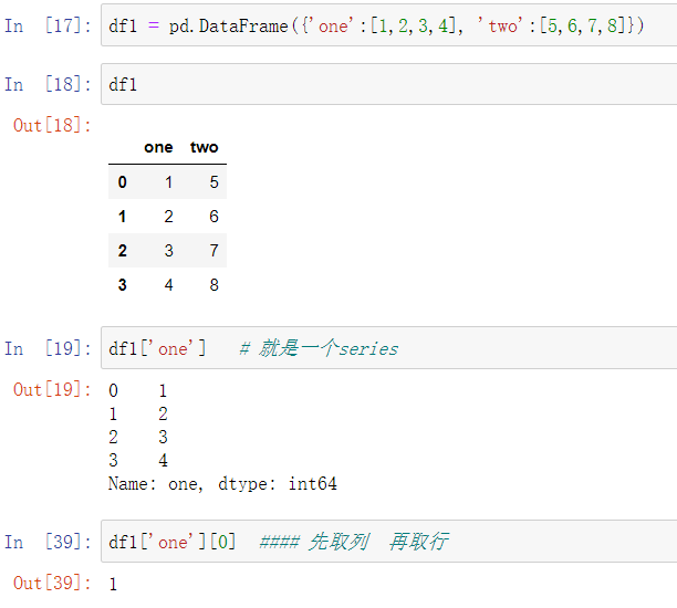
索引与切片
# 索引与切片
df2 = pd.DataFrame({'one':pd.Series([1,2,3],index=['a','b','c']),'two':pd.Series([1,2,3,4],index=['b','a','c','d'])})
print(df2)  # 因为一列series为同一类型,NaN为浮点型,所以整列为浮点型
'''
   one  two
a  1.0    2
b  2.0    1
c  3.0    3
d  NaN    4
'''
print(df2['one']['a'])  # 必须先列后行     1.0
print(df2.loc['a','one'])   # 用标签的方式取值,不容易出整数索引的错,先行后列        1.0
print(df2.loc['a',])   # 显示一行,等同于df2.loc['a',]
'''
one    1.0
two    2.0
Name: a, dtype: float64
'''
print(df2.loc[['a','c'],:]) # 截取a,c两行
'''
   one  two
a  1.0    2
c  3.0    3
'''
print(df2.loc[['a','c'],'two'])
'''
a    2
c    3
Name: two, dtype: int64
'''
常用处理方式:
读取csv格式文件
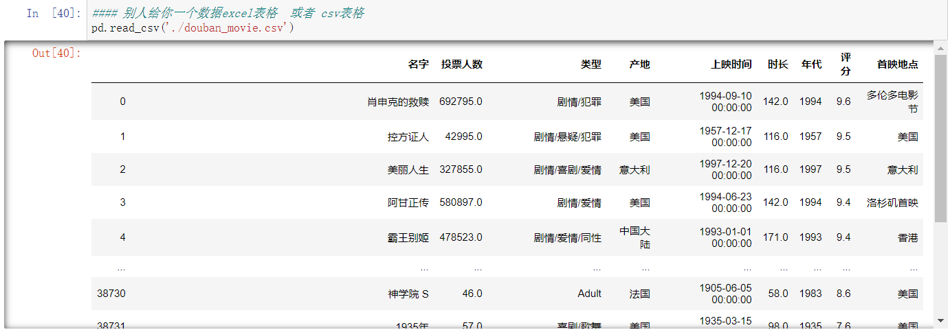
read_csv方法 默认分隔符为逗号
read_table方法 默认分隔符为制表符, 键盘上的tab键
自己写一个test1.csv文件,csv本质是以逗号分隔,内容为
,a,b,c
0,1,2,3
1,4,5,6
2,7,8,9
print(pd.read_csv('test1.csv')) # 读取该文件,在原基础上一列,作为行索引
''' 第一个为空,显示为Unnamed: 0
   Unnamed: 0  a        date  c
0           0  1  2007-02-02  3
1           1  4  2007-02-05  6
2           2  7  2007-02-08  9
'''
print(pd.read_csv('test1.csv',index_col=0)) # 以第一列作为列索引
'''
   a        date  c
0  1  2007-02-02  3
1  4  2007-02-05  6
2  7  2007-02-08  9
'''
print(pd.read_csv('test1.csv',index_col='date'))   # 以date列为列索引,注此处的索引是字符串,而非时间对象
'''
            Unnamed: 0  a  c
date
2007-02-02           0  1  3
2007-02-05           1  4  6
2007-02-08           2  7  9
'''
# parse_dates=True表示把表里所有能解释成时间序列的列都解释出来
df = pd.read_csv('test1.csv',index_col='date',parse_dates=True)
print(df.index) # DatetimeIndex(['2007-02-02', '2007-02-05', '2007-02-08'], dtype='datetime64[ns]', name='date', freq=None)
# parse_dates里也可以传入列表,表示哪些列要解释成时间序列
df = pd.read_csv('test1.csv',index_col='date',parse_dates=['date'])
print(df.index) # DatetimeIndex(['2007-02-02', '2007-02-05', '2007-02-08'], dtype='datetime64[ns]', name='date', freq=None)

# 添加列索引
print(pd.read_csv('test1.csv',header=None)) # 自动创建列索引
'''
     0  1           2  3
0  NaN  a        date  c
1  0.0  1  2007-02-02  3
2  1.0  4  2007-02-05  6
3  2.0  7  2007-02-08  9
'''
print(pd.read_csv('test1.csv',header=None,names=list('abcd')))  # names属性中写入列表
'''
     a  b           c  d
0  NaN  a        date  c
1  0.0  1  2007-02-02  3
2  1.0  4  2007-02-05  6
3  2.0  7  2007-02-08  9
'''
print(pd.read_csv('test1.csv',header=None,names=list('abcd'),skiprows=[1,2]))   # 跳过1,2两行
'''
     a  b           c  d
0  NaN  a        date  c
1  2.0  7  2007-02-08  9
'''
当表格中有None等数据,会连累其他数据变为object
# 因为none类型变为object
print(df[1])    # Name: 2, dtype: object
print(df[1][1]) # 1
print(type(df[1][1])) # <class 'str'> 因为none无法解释,所以这一列变为字符串
# 解决方法,指定字符串变为NaN
print(pd.read_csv('test1.csv',header=None,na_values=['None'])) # 把特定字符解释为NaN
把数据保存为csv文件
df2 = pd.DataFrame({'one':pd.Series([1,2,3],index=['a','b','c']),'two':pd.Series([1,2,3,4],index=['b','a','c','d'])})
print(df2)
'''
   one  two
a  1.0    2
b  2.0    1
c  3.0    3
d  NaN    4
'''
df2.to_csv('test2.csv') # 缺失的值自动变为空
 test2.csv文件
常用属性
- index 获取索引
- T 转置
- columns 获取列索引
- values 获取值数组
- describe() 获取快速统计
df2 = pd.DataFrame({'one':pd.Series([1,2,3],index=['a','b','c']),'two':pd.Series([1,2,3,4],index=['b','a','c','d'])})
print(df2)  # 因为一列series为同一类型,NaN为浮点型,所以整列为浮点型
'''
   one  two
a  1.0    2
b  2.0    1
c  3.0    3
d  NaN    4
'''
print(df2.index)  # 返回行索引
# Index(['a', 'b', 'c', 'd'], dtype='object')
print(df2.values)   # 返回值数组
'''
[[ 1.  2.]
 [ 2.  1.]
 [ 3.  3.]
 [nan  4.]]
'''
print(df2.T)    # 因为一列series为同一类型,转置后每列都有浮点型,全部转为浮点型
'''
       a    b    c    d
one  1.0  2.0  3.0  NaN
two  2.0  1.0  3.0  4.0
'''
print(df2.columns)  # 获取列索引
# Index(['one', 'two'], dtype='object')
print(df2.describe())   # 获取快速统计
'''
       one       two
count  3.0  4.000000    个数
mean   2.0  2.500000    平均值
std    1.0  1.290994    标准差
min    1.0  1.000000    最小值
25%    1.5  1.750000    1/4位数
50%    2.0  2.500000    中位数
75%    2.5  3.250000    3/4位数
max    3.0  4.000000    最大值
'''
数据对齐(相加)
df2 = pd.DataFrame({'one':pd.Series([1,2,3],index=['a','b','c']),'two':pd.Series([1,2,3,4],index=['b','a','c','d'])})
print(df2)  # 因为一列series为同一类型,NaN为浮点型,所以整列为浮点型
'''
   one  two
a  1.0    2
b  2.0    1
c  3.0    3
d  NaN    4
'''
df = pd.DataFrame({'two':[1,2,3,4],'one':[4,5,6,7]},index=['c','d','b','a'])
print(df)
'''
   two  one
c    1    4
d    2    5
b    3    6
a    4    7
'''
print(df + df2) # 运算时行和列都要对齐
'''
   one  two
a  8.0    6
b  8.0    4
c  7.0    4
d  NaN    6
'''
缺失值处理
# 缺失数据处理
import pandas as pd
df2 = pd.DataFrame({'one':pd.Series([1,2,3],index=['a','b','c']),'two':pd.Series([1,2,3,4],index=['b','a','c','d'])})
'''
   one  two
a  1.0    2
b  2.0    1
c  3.0    3
d  NaN    4
'''
print(df2.fillna(0))    # 把缺失值设置为0
'''
   one  two
a  1.0    2
b  2.0    1
c  3.0    3
d  0.0    4
'''
print(df2.dropna())     # 把缺失值整个一行删除
'''
   one  two
a  1.0    2
b  2.0    1
c  3.0    3
'''
import numpy as np
df2.loc['d','two'] = np.nan # 改为缺失值
df2.loc['c','two'] = np.nan # 改为缺失值
print(df2)
'''
   one  two
a  1.0  2.0
b  2.0  1.0
c  3.0  NaN
d  NaN  NaN
'''
print(df2.dropna(how='all'))    # 删除整行都是缺失值NaN的行,how默认参数是any
'''
   one  two
a  1.0  2.0
b  2.0  1.0
c  3.0  NaN
'''

# 以列为单位删除
df = pd.DataFrame({'one':pd.Series([1,2,3],index=['a','b','c']),'two':pd.Series([1,2,3,4],index=['b','a','c','d'])})
'''
   one  two
a  1.0    2
b  2.0    1
c  3.0    3
d  NaN    4
'''
print(df.dropna(axis=1))    # axis代表轴,默认0代表行。1代表列
'''
   two
a    2
b    1
c    3
d    4
'''
常用方法
- mean(axis=0) 对列(行)求平均值
- sum(axis=1) 对列(行)求和
- sort_index(axis,...,ascending) 对列(行)索引排序
- sort_values(by,axis,ascending) 按某一列(行)的值排序
- NumPy的通用函数同样使用与pandas
# pandas常用函数
df = pd.DataFrame({'one':pd.Series([1,2,3],index=['a','b','c']),'two':pd.Series([1,2,3,4],index=['b','a','c','d'])})
'''
   one  two
a  1.0    2
b  2.0    1
c  3.0    3
d  NaN    4
'''
print(df.mean())    # 平均数,返回长度为2的series对象
'''
one    2.0
two    2.5
dtype: float64
'''
print(df.mean(axis=1))  # 按每行求平均值
'''
a    1.5
b    1.5
c    3.0
d    4.0
dtype: float64
'''
print(df.sum()) # 按列求和
'''
one     6.0
two    10.0
'''
print(df.sum(axis=1))   # 按行求和
'''
a    3.0
b    3.0
c    6.0
d    4.0
'''
# 排序
# 注意所有排序NaN的值都不参与排序放在最后
print(df.sort_values(by='two')) # 按第二列正序排列
'''
   one  two
b  2.0    1
a  1.0    2
c  3.0    3
d  NaN    4
'''
print(df.sort_values(by='two',ascending=False)) # ascending升序为false,按第二列倒序排列
print(df.sort_values(by='a',ascending=False,axis=1)) # 按行排序,倒叙
'''
   two  one
a    2  1.0
b    1  2.0
c    3  3.0
d    4  NaN
'''
print(df.sort_index())  # 按标签进行排序
print(df.sort_index(ascending=False))   # 按标签进行降序
'''
   one  two
d  NaN    4
c  3.0    3
b  2.0    1
a  1.0    2
'''
print(df.sort_index(ascending=False,axis=1))    # 按列标签进行降序
'''
   two  one
a    2  1.0
b    1  2.0
c    3  3.0
d    4  NaN
'''
dateutil时间处理
import dateutil # 安装pandas自动安装的库
print(dateutil.parser.parse('2019-07-17'))  # 可以解析各种日期格式    2019-07-17 00:00:00
print(dateutil.parser.parse('2001-JAN-01')) # 2001-01-01 00:00:00
时间对象
# pandas批量把时间装换成时间对象
print(pd.to_datetime(['2001-01-01','2010/Feb/02']))
# DatetimeIndex(['2001-01-01', '2010-02-02'], dtype='datetime64[ns]', freq=None)

# pandas生成时间对象
print(pd.date_range('2010-01-01','2010-5-1'))   # 指定起始和终点   DatetimeIndex可以当作Dataframe或者series的索引
'''
DatetimeIndex(['2010-01-01', '2010-01-02', '2010-01-03', '2010-01-04',
               '2010-01-05', '2010-01-06', '2010-01-07', '2010-01-08',
               '2010-01-09', '2010-01-10',
               ...
               '2010-04-22', '2010-04-23', '2010-04-24', '2010-04-25',
               '2010-04-26', '2010-04-27', '2010-04-28', '2010-04-29',
               '2010-04-30', '2010-05-01'],
              dtype='datetime64[ns]', length=121, freq='D')
'''
# print(pd.date_range('2010-01-01',periods=60))   # 指定起始和长度
print(pd.date_range('2010-01-01',periods=60,freq='H'))   # 频率为小时
'''
DatetimeIndex(['2010-01-01 00:00:00', '2010-01-01 01:00:00',
               '2010-01-01 02:00:00', '2010-01-01 03:00:00',
               '2010-01-01 04:00:00', '2010-01-01 05:00:00',
               '2010-01-01 06:00:00', '2010-01-01 07:00:00',
               ...
'''
print(pd.date_range('2010-01-01',periods=60,freq='W'))   # 频率为周,默认输出每周日
'''
...
                '2011-01-30', '2011-02-06', '2011-02-13', '2011-02-20'],
              dtype='datetime64[ns]', freq='W-SUN')    每周日输出
'''
print(pd.date_range('2010-01-01',periods=60,freq='W-MON'))   # 频率为周,输出每周一
print(pd.date_range('2010-01-01',periods=60,freq='B'))  # B代表business,非周六周日
print(pd.date_range('2010-01-01',periods=60,freq='1h20min'))  # 间隔为1小时20分钟
print(pd.date_range('2010-01-01',periods=60,freq='B')[0])   # 2010-01-01 00:00:00
print(type(pd.date_range('2010-01-01',periods=60,freq='B')[0])) # <class 'pandas._libs.tslibs.timestamps.Timestamp'>
Pandas时间序列Series(切片, 索引)
# pandas时间序列
# DatetimeIndex可以当作Dataframe或者series的索引
sr = pd.Series(np.arange(100),index=pd.date_range('2017-01-01',periods=100))
print(sr)
'''
2017-01-01     0
2017-01-02     1
2017-01-03     2
2017-01-04     3
...
'''
print(sr.index) # 输出DatetimeIndex对象的索引
print(sr['2017-03'])    # 显示2017年3月所有
'''
2017-03-01    59
2017-03-02    60
2017-03-03    61
...
'''
print(sr['2017':'2018-03']) # 时间切片
print(sr.resample('W').sum())   # resample重新采样,按周求和
'''
2017-01-01      0
2017-01-08     28
2017-01-15     77
2017-01-22    126
...
'''
print(sr.resample('M').mean())  # 按每月求平均值
# truncate方法截断,可以用切片,意义不大
print(sr.truncate(before='2017-02-03')) # 截断2017-02-03之前的部分,只取后面的部分,包括2017-02-03
'''
Freq: M, dtype: float64
2017-02-03    33
2017-02-04    34
2017-02-05    35
...
'''
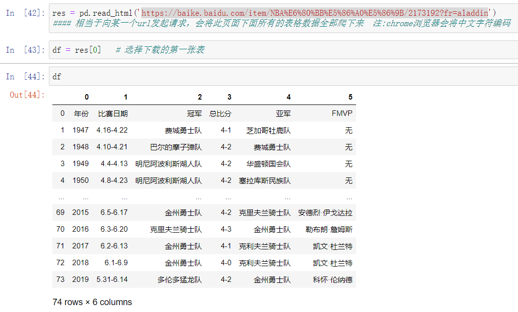
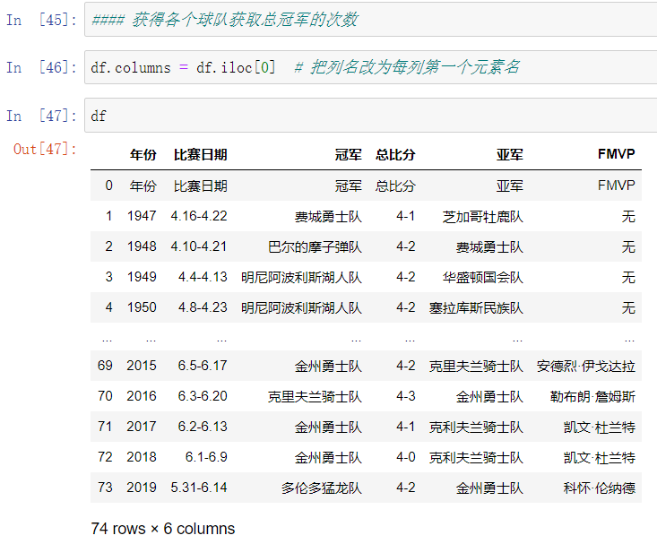
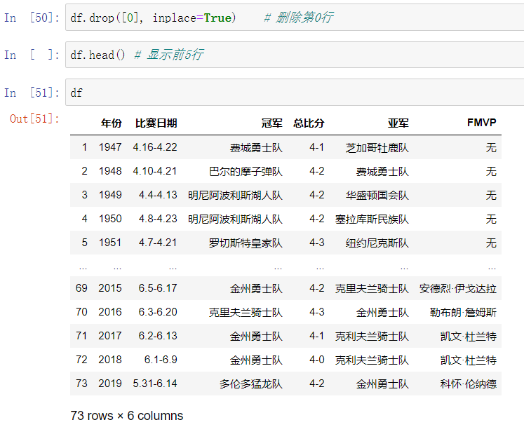
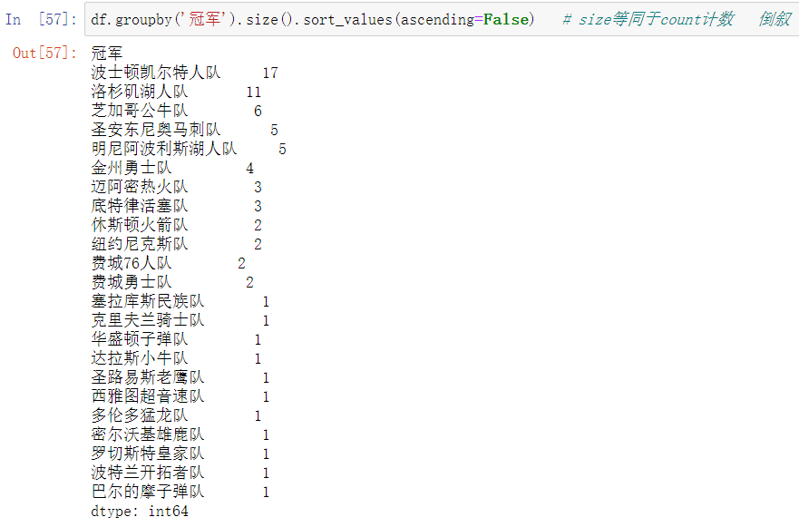
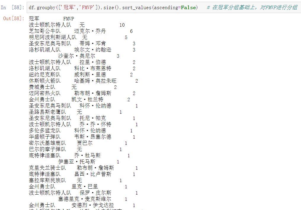
读取html表格数据
NBA总冠军百度百科 注:chrome浏览器会自动把中文转化为编码
https://baike.baidu.com/item/NBA%E6%80%BB%E5%86%A0%E5%86%9B/2173192?fr=aladdin