自己利用python动手实现手写数字识别
在这里我自己用python写了识别手写0-9数字的程序,利用了逻辑回归方法以及正则化,one-vs-all的技巧(如果不知道这两个概念的可以看一下我以前发的博客)。
数据准备和环境
这里的数据是一个5000 × 400的矩阵,意思就是有5000张图片而每一张都是20*20的灰度图片(这里是被拉伸成了一行),y就是标签是个5000×1的矩阵,取值范围为1-10,这里10就代表0。而且数据是以mat的形式存储的(matlab存文件就是这个形式)。
这里为了方便矩阵运算,读取文件和画图需要引入numpy,matplot,scipy三个库。
主程序(调度用的)
# ================== Multi-class Classification | part 1: one vs all ========================
from scipy.io import loadmat  # read matfile
import numpy as np
import displayData
import lrCostFunction
import oneVsAll
import Predict
import matplotlib.pyplot as plt
import predictOneVsAll
# ================== load Data =============================================================
data = loadmat("../machine-learning-ex3/ex3/ex3data1.mat")
x_data = data["X"]   # x_data here is a 5000 * 400 matrix (5000 training examples, 20 * 20 grid of pixel is unrolled into 4000-deminsional vector
y_data = data.get("y")  # y_data here is a 5000 * 1 matrix(label)
# hint : must transpose the data to get the oriented data
x_data = np.array([im.reshape((20, 20)).T for im in x_data])
x_data = np.array([im.reshape((400, )) for im in x_data])
print(y_data)
# can use data.key() and debugging to get this information
# ================== load end ==============================================================
# set some params
input_layer_size = 400
num_labels = 10
# ================== visualize the data ====================================================
rand = np.random.randint(0, 5000, (100, ))  # [0, 5000)
displayData.data_display(x_data[rand, :])   # get 100 images randomly
# ======================= Test case for lrCostFunction =============================
theta_t = np.array([-2, -1, 1, 2])
t = np.linspace(1, 15, 15) / 10
t = t.reshape((3, 5))
x_t = np.column_stack((np.ones((5, 1)), t.T))
y_t = np.array([1, 0, 1, 0, 1])
l_t = 3
cost = lrCostFunction.cost_reg(theta_t, x_t, y_t, l_t)
grad = lrCostFunction.grad_reg(theta_t, x_t, y_t, l_t)
print("cost is {}".format(cost))
print("expected cost is 2.534819")
print("grad is {}".format(grad))
print("expected grad is 0.146561 -0.548558 0.724722 1.398003")
# ============================ test end =============================================
# ============================ one vs all:predict ===========================================
l = 0.1
theta = oneVsAll.one_vs_all(x_data, y_data, l, num_labels)
result = Predict.pred_lr(theta, x_data[1500, :])
np.set_printoptions(precision=2, suppress=True)  # don't use  scientific notation
print("this number is {}".format(result))  # 10 here is 0
plt.imshow(x_data[1500, :].reshape((20, 20)), cmap='gray', vmin=-1, vmax=1)
plt.show()
accuracy = predictOneVsAll.pred_accuracy(theta, x_data, y_data)
print("test 5000 images, accuracy is {:%}".format(accuracy))
# ============================ predict  end ======================================================
数据可视化(displayData)
这里需要说明的是这里的x_data数据需要把其还原成20*20的矩阵再转置才能画出摆放方向正确的图像。
import numpy as np
import matplotlib.pyplot as plt


def data_display(data, image_width=20):
    # compute image_height
    m, n = data.shape
    image_height = n / image_width
    # compute rows and cols
    display_rows = np.round(np.sqrt(m))
    display_cols = m / display_rows
    # set image padding
    pad = 1
    rows_pixel = np.ceil(display_rows * image_height + (display_rows + 1) * pad)
    cols_pixel = np.ceil(display_cols * image_width + (display_cols + 1) * pad)
    rows_pixel = rows_pixel.astype(np.int64)
    cols_pixel = cols_pixel.astype(np.int64)
    # initialize display matrix
    display_matrix = -np.ones((rows_pixel, cols_pixel))
    # the first pixel of every image is 1+(image_width+pad)*(n-1) or 1+(image_height+pad)*(n-1)
    for i in range(data.shape[0]):
        image_data = data[i, :].reshape((int(image_width), int(image_height)))
        row_index = np.floor(i / display_cols)
        cols_index = i % display_cols
        row_position = pad+(image_height+pad)*row_index
        cols_position = pad+(image_width+pad)*cols_index
        display_matrix[int(row_position):int(row_position+image_height), int(cols_position):int(cols_position+image_width)] = image_data[:, :]
    plt.imshow(display_matrix, cmap='gray', vmin=-1, vmax=1)
    plt.show()
我这里在展示手写图片的时候,只需要一次循环就可以完成,主要的技巧就是利用等差数列求出来每张图片左上角的像素在大矩阵中的位置即可比较方便地完成图片展示。
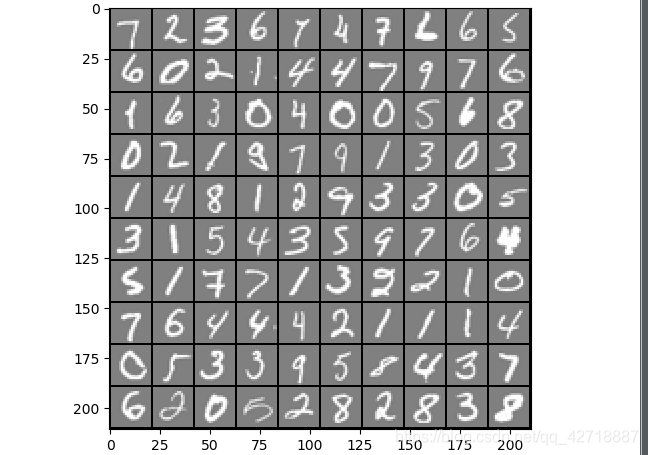
这就是展示出来的样子,可以调节pad来控制图片的黑边间隔。
求损失和梯度的程序(lrCostFunction)
import numpy as np


def sigmoid(x):
    return 1 / (1 + np.exp(-x))


def cost_reg(theta, x_data, y_data, l):
    m, n = x_data.shape
    theta = theta.reshape((-1, 1))
    y_data = y_data.reshape((-1, 1))
    hx = sigmoid(np.dot(x_data, theta))
    ln_h = np.log(hx)
    part1 = -np.dot(ln_h.T, y_data) / m
    ln_1h = np.log(1 - hx)
    part2 = -np.dot(ln_1h.T, 1-y_data) / m
    #   don't do that : theta[0, 0] = 0  # don't penalize theta0
    reg = l * np.dot(theta[1:, :].T, theta[1:, :]) / (2 * m)
    return (part1+part2+reg).flatten()


def grad_reg(theta, x_data, y_data, l):
    m, n = x_data.shape
    theta_tempt = theta.reshape((-1, 1)).copy()
    y_data = y_data.reshape((-1, 1))
    hx = sigmoid(np.dot(x_data, theta_tempt))
    theta_tempt[0, 0] = 0  # don't penalize theta0
    part1 = np.dot(x_data.T, hx - y_data)
    part2 = l * theta_tempt
    return ((part1+part2) / m).flatten()
这里比较坑的一个地方就是第二个函数求梯度的时候一定要进行拷贝,不然的话直接对这个引用进行操作将其[0,0]的元素赋值为0就会导致外部的theta改变。
一对多训练(oneVsAll)
import numpy as np
import fmincg

def one_vs_all(x_data, y_data, l, num_labels):
    # initialize some params
    m, n = x_data.shape
    x_data = np.column_stack((np.ones((m, 1)), x_data))
    # initialize initial_theta
    initial_thata = np.zeros((num_labels, n+1))
    theta = fmincg.fmincg(initial_thata, x_data, y_data, l, num_labels)
    return theta
这里就是一对多的训练,我们要进行k分类就需要训练出k个分类器。
批量优化theta(oneVsAll)
import scipy.optimize as op
import numpy as np
import lrCostFunction


def fmincg(theta, x_data, y_data, l, num_labels):
    for i in range(num_labels):
        y_tempt = y_data.copy()  # hint: must copy !
        # pre-treat
        pos = np.where(y_data == i)
        neg = np.where(y_data != i)
        if i == 0:
            pos = np.where(y_data == 10)
            neg = np.where(y_data != 10)
        y_tempt[pos] = 1
        y_tempt[neg] = 0
        result = op.minimize(lrCostFunction.cost_reg, theta[i, :].T, args=(x_data, y_tempt, l), method="TNC", jac=lrCostFunction.grad_reg)
        print("{} : {}".format(i, result.success))
        theta[i, :] = result.x
    return theta
这里就会返回一个10*401(10个分类器)的theta矩阵,这里利用scipy中比梯度下降更快的高级算法,这个算法一般不会需要自己去实现,除非对自己的数值计算很有信心。当然我在github上面也放上了自己实现的梯度下降算法也可以来优化theta,但是速度肯定要慢一些。
预测(Predict)
import numpy as np
import lrCostFunction


def pred_lr(theta, x_data):
    x_data = x_data.reshape((1, -1))
    x_data = np.column_stack((np.ones((1, 1)), x_data))
    result = lrCostFunction.sigmoid(x_data @ theta.T)
    predict = np.argmax(result.flatten())
    if predict == 0:
        predict = 10
    return predict
这就是预测的代码。
精度验证(predictOneVsAll)
import Predict

def pred_accuracy(theta, x_data, y_data):
    right_num = 0
    m, _ = x_data.shape
    for i in range(m):
        pred = Predict.pred_lr(theta, x_data[i, :])
        if pred == y_data[i, :]:
            right_num += 1
    return right_num / m
还有神经网络版本的实现,我就放在我的github上面了。
https://github.com/lsl1229840757/machine_learning/tree/master/programming_ex3/ex3