Recurrent Neural Networks
Recurrent neural networks are networks with loops in them, allowing information to persist.
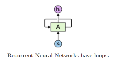
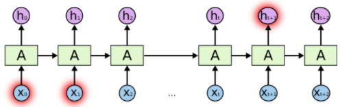
A recurrent neural network can be thought of as multiple copies of the same network, each passing a message to a successor. Consider what happens if we unroll the loop:

This chain-like nature reveals that recurrent neural networks are intimately related to sequences and lists. They’re the natural architecture of neural network to use for such data.
“LSTMs,” a very special kind of recurrent neural network which works, for many tasks, much much better than the standard version. Almost all exciting results based on recurrent neural networks are achieved with them.
One of the appeals of RNNs is the idea that they might be able to connect previous information to the present task, such as using previous video frames might inform the understanding of the present frame. however,It’s entirely possible for the gap between the relevant information and the point where it is needed to become very large.Unfortunately, as that gap grows, RNNs become unable to learn to connect the information.
LSTM Networks
Long Short Term Memory networks – usually just called “LSTMs” – are a special kind of RNN, capable of learning long-term dependencies.
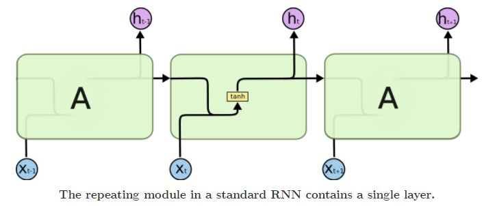
All recurrent neural networks have the form of a chain of repeating modules of neural network. In standard RNNs, this repeating module will have a very simple structure, such as a single tanh layer.
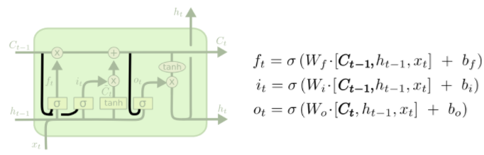
LSTMs also have this chain like structure, but the repeating module has a different structure. Instead of having a single neural network layer, there are four, interacting in a very special way.

一些记号:
The core idea behind LSTMs
The key to LSTMs is the cell state, the horizontal line running through the top of the diagram.
The cell state is kind of like a conveyor belt. It runs straight down the entire chain, with only some minor linear interactions. It’s very easy for information to just flow along it unchanged.

The LSTM does have the ability to remove or add information to the cell state, carefully regulated by structures called gates.
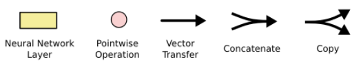
Gates are a way to optionally let information through. They are composed out of a sigmoid neural net layer and a pointwise multiplication operation.
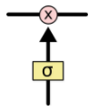
The sigmoid layer outputs numbers between zero and one, describing how much of each component should be let through. A value of zero means “let nothing through,” while a value of one means “let everything through!”
step-by-step LSTM Walk Through
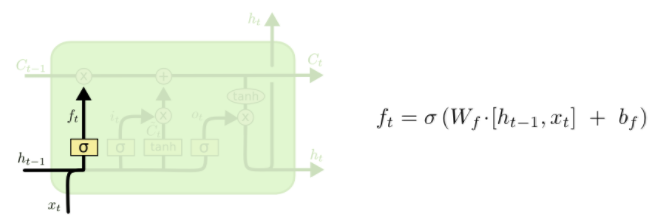
The first step in our LSTM is to decide what information we’re going to throw away from the cell state. This decision is made by a sigmoid layer called the “forget gate layer.” It looks at (h_{t-1}) and (x_t), and outputs a number between (0) and (1) for each number in the cell state (C_{t-1}). A (1) represents “completely keep this” while a (0) represents “completely get rid of this.”
Let’s go back to our example of a language model trying to predict the next word based on all the previous ones. In such a problem, the cell state might include the gender of the present subject, so that the correct pronouns can be used. When we see a new subject, we want to forget the gender of the old subject.
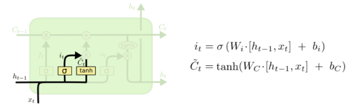
The next step is to decide what new information we’re going to store in the cell state. This has two parts. First, a sigmoid layer called the “input gate layer” decides which values we’ll update. Next, a tanh layer creates a vector of new candidate values, ( ilde{C}_t), that could be added to the state. In the next step, we’ll combine these two to create an update to the state.
In the example of our language model, we’d want to add the gender of the new subject to the cell state, to replace the old one we’re forgetting.
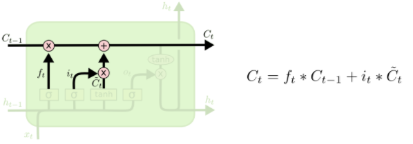
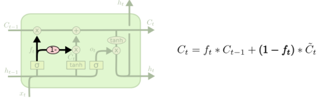
It’s now time to update the old cell state, (C_{t-1}), into the new cell state (C_t). The previous steps already decided what to do, we just need to actually do it.
We multiply the old state by (f_t), forgetting the things we decided to forget earlier. Then we add (i_t* ilde{C}_t). This is the new candidate values, scaled by how much we decided to update each state value.
In the case of the language model, this is where we’d actually drop the information about the old subject’s gender and add the new information, as we decided in the previous steps.
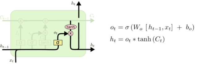
Finally, we need to decide what we’re going to output. This output will be based on our cell state, but will be a filtered version. First, we run a sigmoid layer which decides what parts of the cell state we’re going to output. Then, we put the cell state through ( anh) (to push the values to be between (-1) and (1)) and multiply it by the output of the sigmoid gate, so that we only output the parts we decided to.
For the language model example, since it just saw a subject, it might want to output information relevant to a verb, in case that’s what is coming next. For example, it might output whether the subject is singular or plural, so that we know what form a verb should be conjugated into if that’s what follows next.
Variants on Long Short Term Memory
What I’ve described so far is a pretty normal LSTM. But not all LSTMs are the same as the above. In fact, it seems like almost every paper involving LSTMs uses a slightly different version. The differences are minor, but it’s worth mentioning some of them.
One popular LSTM variant, introduced by Gers & Schmidhuber (2000), is adding “peephole connections.” This means that we let the gate layers look at the cell state.
The above diagram adds peepholes to all the gates, but many papers will give some peepholes and not others.
Another variation is to use coupled forget and input gates. Instead of separately deciding what to forget and what we should add new information to, we make those decisions together. We only forget when we’re going to input something in its place. We only input new values to the state when we forget something older.
http://colah.github.io/posts/2015-08-Understanding-LSTMs/
具体应用见 http://book.paddlepaddle.org/index.cn.html 中情感分析和语义角色标注两个章节
全连接神经网络和卷积神经网络只能单独的去处理一个个的输入,前一个输入和后一个输入是完全没有关系的。但是,某些任务需要能够更好的处理序列的信息,即前面的输入和后面的输入是有关系的。比如,当我们在理解一句话意思时,孤立的理解这句话的每个词是不够的,我们需要处理这些词连接起来的整个序列;当我们处理视频的时候,我们也不能只单独的去分析每一帧,而要分析这些帧连接起来的整个序列。
基本循环神经网络
下图是一个简单的循环神经网络如,它由输入层、一个隐藏层和一个输出层组成:

将上图展开,得到:
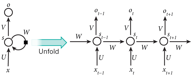
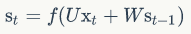
这个网络在$t$时刻接收到输入$X_t$之后,隐藏层的值是$S_t$,输出值是$O_t$。关键一点是,$S_t$的值不仅仅取决于$X_t$,还取决于$S_{t-1}$。我们可以用下面的公式来表示循环神经网络的计算方法:
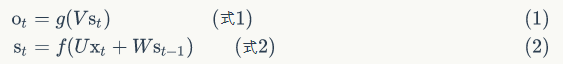
如果反复把式2带入到式1,我们将得到:

从上面可以看出,循环神经网络的输出值$O_t$,是受前面历次输入值影响的,这就是为什么循环神经网络可以往前看任意多个输入值的原因。
双向循环神经网络
对于语言模型来说,很多时候光看前面的词是不够的,比如下面这句话:
我的手机坏了,我打算____一部新手机。
可以想象,如果我们只看横线前面的词,手机坏了,那么我是打算修一修?换一部新的?还是大哭一场?这些都是无法确定的。但如果我们也看到了横线后面的词是『一部新手机』,那么,横线上的词填『买』的概率就大得多了。
在上一小节中的基本循环神经网络是无法对此进行建模的,因此,我们需要双向循环神经网络,如下图所示:
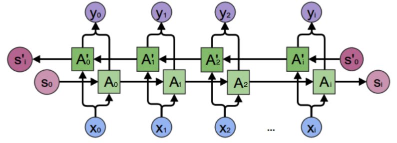
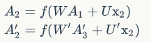
考虑上图中$y_2$的计算,从上图可以看出,双向卷积神经网络的隐藏层要保存两个值,一个A参与正向计算,另一个值A'参与反向计算。最终的输出值$y_2$取决于$A_2$ 和 $A_2^`$。其计算方法为:

从上面三个公式我们可以看到,正向计算和反向计算不共享权重,也就是说U和U'、W和W'、V和V'都是不同的权重矩阵。
深度循环神经网络
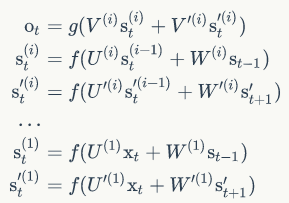
前面我们介绍的循环神经网络只有一个隐藏层,我们当然也可以堆叠两个以上的隐藏层,这样就得到了深度循环神经网络。如下图所示:
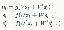
我们把第i个隐藏层的值表示为$S_t^{i}$、$S_t^{'i}$,则深度循环神经网络的计算方式可以表示为:
循环神经网络的训练算法:BPTT
BPTT算法是针对循环层的训练算法,它的基本原理和BP算法是一样的,也包含同样的三个步骤:
1、前向计算每个神经元的输出值;
2、反向计算每个神经元的误差项值,它是误差函数E对神经元j的加权输入的偏导数;
3、计算每个权重的梯度。
最后再用随机梯度下降算法更新权重。
循环层如下图所示:

前向计算
对循环层进行前向计算:
我们假设输入向量x的维度是m,输出向量s的维度是n,则矩阵U的维度是n * n,矩阵W的维度是n * m。
误差项的计算
BTPP算法将第l层t时刻的误差项$delta^l_t$值沿两个方向传播,一个方向是其传递到上一层网络得到$delta^{l-1}_t$,这部分只和权重矩阵U有关;另一个是方向是将其沿时间线传递到初始$t_1$时刻,得到$delta^l_1$,这部分只和权重矩阵W有关。
我们用向量$net_t$表示神经元在t时刻的加权输入,因为:
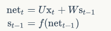
因此:

https://www.zybuluo.com/hanbingtao/note/541458
http://blog.csdn.net/heyongluoyao8/article/details/48636251