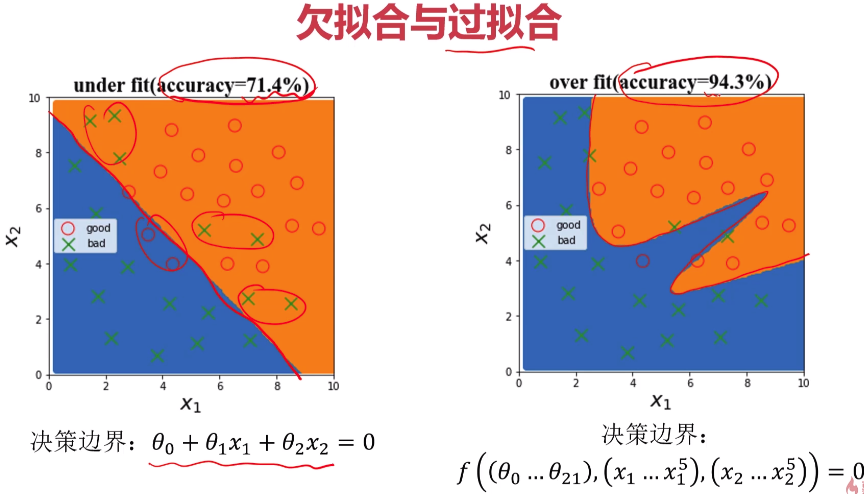
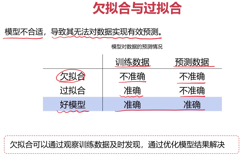
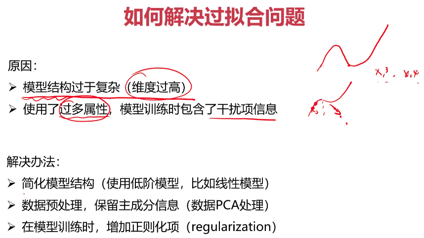
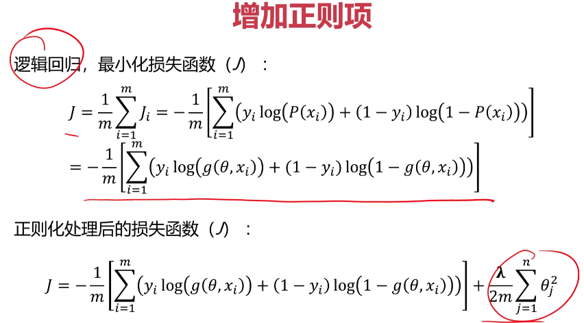
- 过拟合和欠拟合


- 数据分离与混淆矩阵


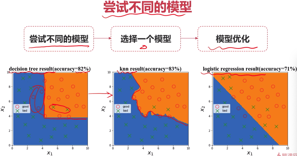
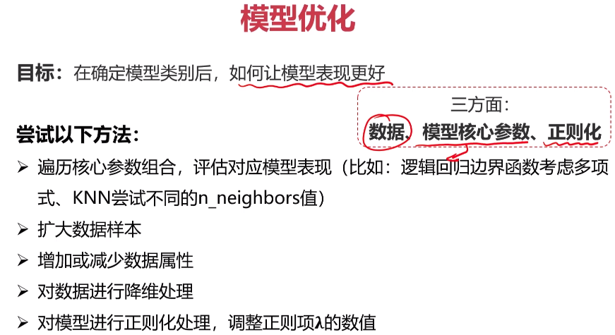
- 模型优化
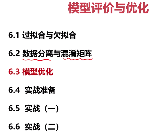


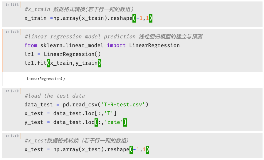
- 实战准备


- 实战一


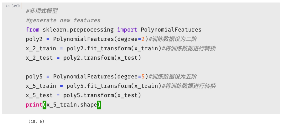

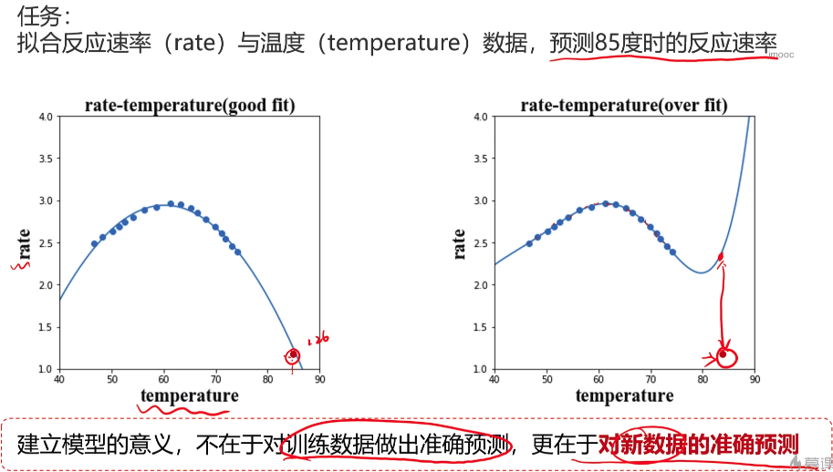
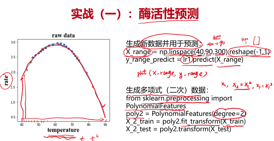
1 #generate new data 建立新数据
2 x_2_range = np.linspace(40,90,300).reshape(-1,1)#最小值40,最大值90,产生300个点;转成300行一列的数组
3 x_2_range = poly2.transform(x_2_range)
4 y_2_range_predict = lr2.predict(x_2_range)
5
6 x_5_range = np.linspace(40,90,300).reshape(-1,1)#最小值40,最大值90,产生300个点;转成300行一列的数组
7 x_5_range = poly5.transform(x_5_range)
8 y_5_range_predict = lr5.predict(x_5_range)


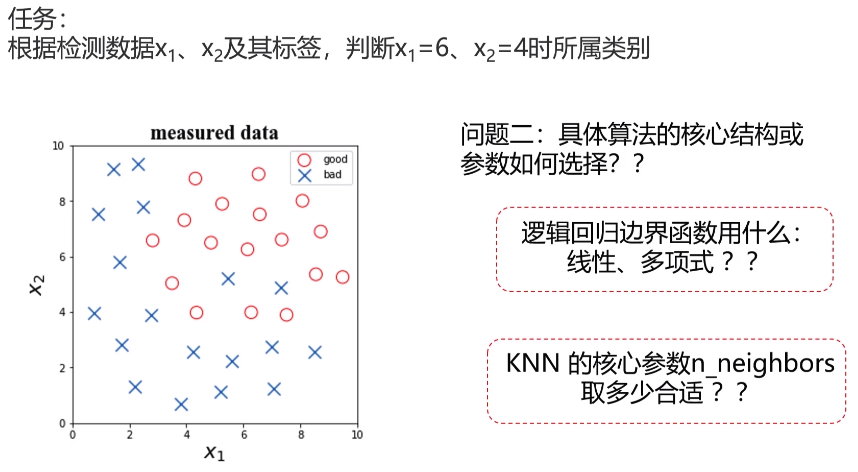
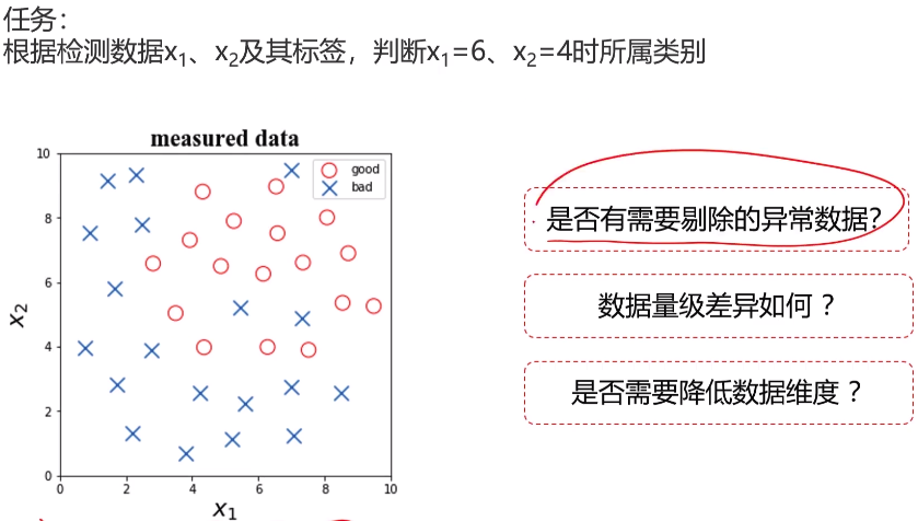
- 实战二

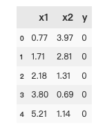
1 #load the data
2 import pandas as pd
3 import numpy as np
4 data = pd.read_csv('data_class_raw.csv')
5 data.head()
1 #define x and y
2 x = data.drop(['y'],axis=1)
3 y = data.loc[:,'y']
4 print(x.shape,y.shape)

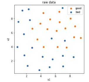
 1 #visualize the data
 2 %matplotlib inline
 3 from matplotlib import pyplot as plt
 4 fig1 = plt.figure(figsize=(5,5))
 5 bad = plt.scatter(x.loc[:,'x1'][y==0],x.loc[:,'x2'][y==0])
 6 good = plt.scatter(x.loc[:,'x1'][y==1],x.loc[:,'x2'][y==1])
 7 plt.legend((good,bad),('good','bad'))
 8 plt.title('raw data')
 9 plt.xlabel('x1')
10 plt.ylabel('x2')
11 plt.show()
1 #anomaly detextion 异常点检测
2 from sklearn.covariance import EllipticEnvelope
3 ad_model = EllipticEnvelope(contamination=0.02)
4 ad_model.fit(x[y==0])
5 y_predict_bad = ad_model.predict(x[y==0])
6 print(y_predict_bad)
[ 1 1 1 1 1 1 1 1 1 1 1 1 1 1 1 1 1 1 -1]
 1 #visualize the data
 2 %matplotlib inline
 3 from matplotlib import pyplot as plt
 4 fig1 = plt.figure(figsize=(5,5))
 5 bad = plt.scatter(x.loc[:,'x1'][y==0],x.loc[:,'x2'][y==0])
 6 good = plt.scatter(x.loc[:,'x1'][y==1],x.loc[:,'x2'][y==1])
 7 plt.scatter(x.loc[:,'x1'][y==0][y_predict_bad==-1],x.loc[:,'x2'][y==0][y_predict_bad==-1],marker='x',s=150)
 8 plt.legend((good,bad),('good','bad'))
 9 plt.title('raw data')
10 plt.xlabel('x1')
11 plt.ylabel('x2')
12 plt.show()

1 data = pd.read_csv('data_class_processed.csv')
2 data.head()
3 #define x and y
4 x = data.drop(['y'],axis=1)
5 y = data.loc[:,'y']
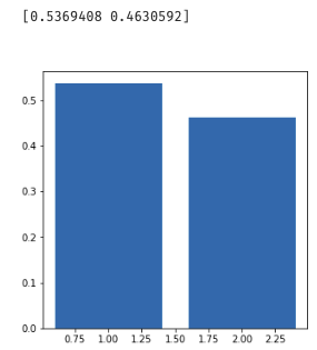
 1 #pca
 2 from sklearn.preprocessing import StandardScaler
 3 from sklearn.decomposition import PCA
 4 x_norm = StandardScaler().fit_transform(x)#标准化处理数据
 5 pca = PCA(n_components=2)
 6 x_reduced = pca.fit_transform(x_norm)
 7 var_ratio = pca.explained_variance_ratio_
 8 print(var_ratio)
 9 fig4 = plt.figure(figsize=(5,5))
10 plt.bar([1,2],var_ratio)
11 plt.show()
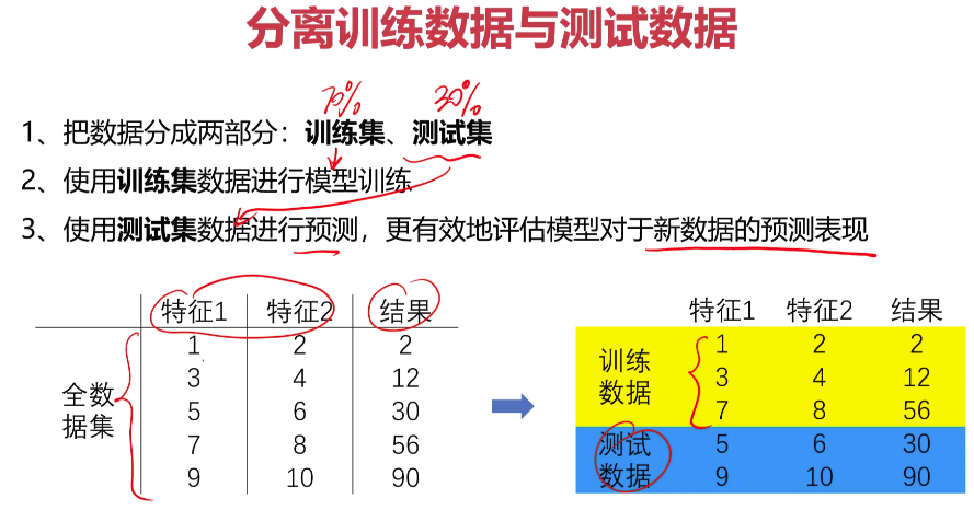
1 #train and test split:random_state=4,test_size=0.4 数据分离
2 from sklearn.model_selection import train_test_split
3 x_train, x_test, y_train, y_test = train_test_split(x,y,random_state=4,test_size=0.4)
4 print(x_train.shape,x_test.shape,x.shape)
 1 #knn model
 2 from sklearn.neighbors import KNeighborsClassifier
 3 knn_10 = KNeighborsClassifier(n_neighbors=10)
 4 knn_10.fit(x_train,y_train)
 5 y_train_predict = knn_10.predict(x_train)
 6 y_test_predict = knn_10.predict(x_test)
 7 #calculate the accuracy
 8 from sklearn.metrics import accuracy_score
 9 accuracy_train = accuracy_score(y_train,y_train_predict)
10 accuracy_test = accuracy_score(y_test,y_test_predict)
11 print('training accuracy:',accuracy_train)
12 print('testing accuracy:',accuracy_test)
training accuracy: 0.9047619047619048
testing accuracy: 0.6428571428571429
1 #visualize the knn result and boundary 2 xx, yy = np.meshgrid(np.arange(0,10,0.05),np.arange(0,10,0.05)) 3 print(yy.shape)
(200, 200)

1 x_range = np.c_[xx.ravel(),yy.ravel()] 2 print(x_range.shape)
(40000, 2)
1 y_range_predict = knn_10.predict(x_range)
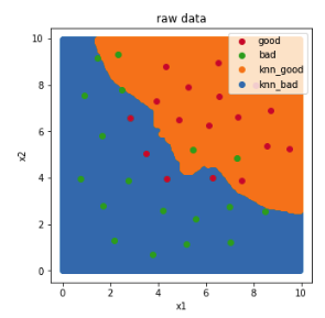
 1 fig4 = plt.figure(figsize=(5,5))
 2 knn_bad = plt.scatter(x_range[:,0][y_range_predict==0],x_range[:,1][y_range_predict==0])
 3 knn_good = plt.scatter(x_range[:,0][y_range_predict==1],x_range[:,1][y_range_predict==1])
 4
 5 bad = plt.scatter(x.loc[:,'x1'][y==0],x.loc[:,'x2'][y==0])
 6 good = plt.scatter(x.loc[:,'x1'][y==1],x.loc[:,'x2'][y==1])
 7 plt.legend((good,bad,knn_good,knn_bad),('good','bad','knn_good','knn_bad'))
 8 plt.title('raw data')
 9 plt.xlabel('x1')
10 plt.ylabel('x2')
11 plt.show()
1 from sklearn.metrics import confusion_matrix 2 cm = confusion_matrix(y_test,y_test_predict) 3 print(cm)
[[4 2]
 [3 5]]
 1 TP = cm[1,1] 2 TN = cm[0,0] 3 FP = cm[0,1] 4 FN = cm[1,0] 5 print(TP,TN,FP,FN)
5 4 2 3
 1 accuracy =(TP+TN)/(TP+TN+FP+FN)#准确率:整体样本中正确样本数的比例
 2 recall = TP/(TP+FP)#Sensitivity 灵敏度(召回率):正样本中,预测正确的比例
 3 specificity = TN/(TN+FP)#特异度:负样本中,预测正确的比例
 4 precision = TP/(TP+FP)#精确率:预测结果为正样本中,预测正确的比例
 5 f1 = 2*precision*recall/(precision + recall)#F1 Score:综合Precision和Recall的喝一喝判断指标
 6 print('准确率:',accuracy)
 7 print('灵敏度:',recall)
 8 print('特异度:',specificity)
 9 print('精确率:',precision)
10 print('F1 Score:',f1)
准确率: 0.6428571428571429
灵敏度: 0.7142857142857143
特异度: 0.6666666666666666
精确率: 0.7142857142857143
F1 Score: 0.7142857142857143
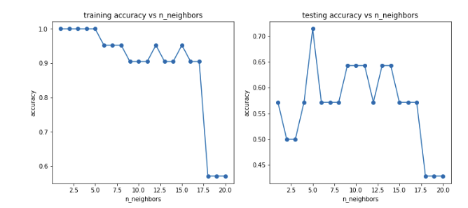
 1 #try different k and calcualte the accuracy for each
 2 n = [i for i in range(1,21)]
 3 accuracy_train = []
 4 accuracy_test = []
 5 for i in n:
 6     knn = KNeighborsClassifier(n_neighbors=i)
 7     knn.fit(x_train,y_train)
 8     y_train_predict = knn.predict(x_train)
 9     y_test_predict = knn.predict(x_test)
10     accuracy_train_i = accuracy_score(y_train,y_train_predict)
11     accuracy_test_i = accuracy_score(y_test,y_test_predict)
12     accuracy_train.append(accuracy_train_i)
13     accuracy_test.append(accuracy_test_i)
14 print(accuracy_train,accuracy_test)
[1.0, 1.0, 1.0, 1.0, 1.0, 0.9523809523809523, 0.9523809523809523, 0.9523809523809523, 0.9047619047619048, 0.9047619047619048, 0.9047619047619048, 0.9523809523809523, 0.9047619047619048, 0.9047619047619048, 0.9523809523809523, 0.9047619047619048, 0.9047619047619048, 0.5714285714285714, 0.5714285714285714, 0.5714285714285714]
[0.5714285714285714, 0.5, 0.5, 0.5714285714285714, 0.7142857142857143, 0.5714285714285714, 0.5714285714285714, 0.5714285714285714, 0.6428571428571429, 0.6428571428571429, 0.6428571428571429, 0.5714285714285714, 0.6428571428571429, 0.6428571428571429, 0.5714285714285714, 0.5714285714285714, 0.5714285714285714, 0.42857142857142855, 0.42857142857142855, 0.42857142857142855]
 1 fig5 = plt.figure(figsize=(12,5))
 2 plt.subplot(121)
 3 plt.plot(n,accuracy_train,marker='o')
 4 plt.title('training accuracy vs n_neighbors')
 5 plt.xlabel('n_neighbors')
 6 plt.ylabel('accuracy')
 7
 8 plt.subplot(122)
 9 plt.plot(n,accuracy_test,marker='o')
10 plt.title('testing accuracy vs n_neighbors')
11 plt.xlabel('n_neighbors')
12 plt.ylabel('accuracy')
13 plt.show()