相关概念:
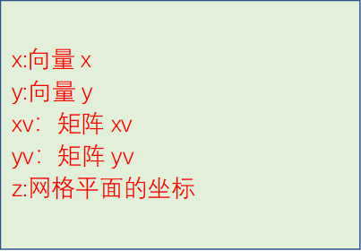
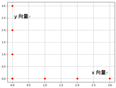
1.x向量和y向量


import numpy as np
import matplotlib.pyplot as plt
x = np.array([[0,1,2,3],
              [0,0,0,0],
              [0,0,0,0],
              [0,0,0,0]])
y = np.array([[0,0,0,0],
              [1,0,0,0],
              [2,0,0,0],
              [3,0,0,0]])
plt.plot(x,y,
         color = 'red',  ##全部点设置红色
         marker='o',     ##形状:实心圆圈
         linestyle = '') ##线性:空  点与点间不连线
plt.grid(True)           ##显示网格
plt.show()
x向量:[0, 1, 2, 3]
y向量:[0, 1, 2, 3]
2.xv和yv矩阵
import numpy as np
import matplotlib.pyplot as plt
x = [0,1,2,3]
y = [0,1,2,3]
print(x)
print(y)
x,y = np.meshgrid(x,y)
print(x)
print(y)
plt.plot(x,y,
         color = 'red',  ##全部点设置红色
         marker='o',     ##形状:实心圆圈
         linestyle = '') ##线性:空  点与点间不连线
plt.grid(True)           ##显示网格
plt.show()
xv坐标矩阵:
[[0 1 2 3]
[0 1 2 3]
[0 1 2 3]
[0 1 2 3]]
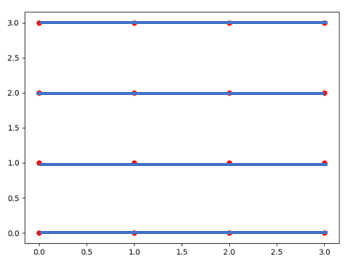
yv坐标矩阵:
[[0 0 0 0]
[1 1 1 1]
[2 2 2 2]
[3 3 3 3]]

z:网格平面坐标

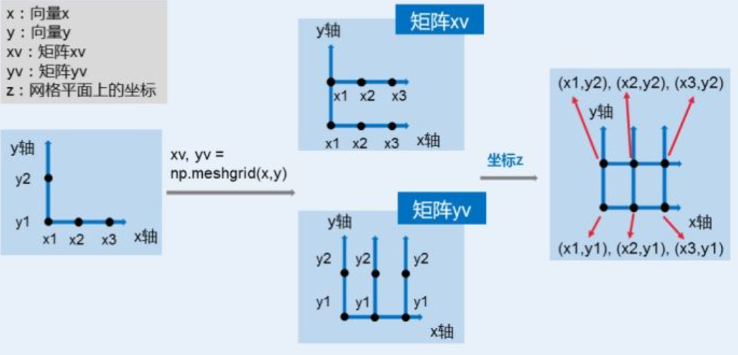
图片来源:https://www.cnblogs.com/lantingg/p/9082333.html
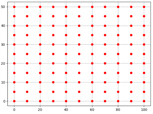
import numpy as np
import matplotlib.pyplot as plt
#调用meshgrid实现以上功能
x = np.linspace(0,100,11)
y = np.linspace(0,50,11)
print(x)
print(y)
x,y = np.meshgrid(x,y)
print('x--meshgrid后的数据',x)
print('y--meshgrid后的数据',y)
plt.plot(x,y,
         color = 'red',  ##全部点设置红色
         marker='o',     ##形状:实心圆圈
         linestyle = '') ##线性:空  点与点间不连线
plt.grid(True)           ##显示网格
plt.show()
'''
x = [  0.  10.  20.  30.  40.  50.  60.  70.  80.  90. 100.]
y = [ 0.  5. 10. 15. 20. 25. 30. 35. 40. 45. 50.]
x--meshgrid后的数据 [将x一维数组,重复11次]
[[  0.  10.  20.  30.  40.  50.  60.  70.  80.  90. 100.]
 [  0.  10.  20.  30.  40.  50.  60.  70.  80.  90. 100.]
 [  0.  10.  20.  30.  40.  50.  60.  70.  80.  90. 100.]
 [  0.  10.  20.  30.  40.  50.  60.  70.  80.  90. 100.]
 [  0.  10.  20.  30.  40.  50.  60.  70.  80.  90. 100.]
 [  0.  10.  20.  30.  40.  50.  60.  70.  80.  90. 100.]
 [  0.  10.  20.  30.  40.  50.  60.  70.  80.  90. 100.]
 [  0.  10.  20.  30.  40.  50.  60.  70.  80.  90. 100.]
 [  0.  10.  20.  30.  40.  50.  60.  70.  80.  90. 100.]
 [  0.  10.  20.  30.  40.  50.  60.  70.  80.  90. 100.]
 [  0.  10.  20.  30.  40.  50.  60.  70.  80.  90. 100.]]
y--meshgrid后的数据 [将y一位数组转置成列,再重复11次]
[[ 0.  0.  0.  0.  0.  0.  0.  0.  0.  0.  0.]
 [ 5.  5.  5.  5.  5.  5.  5.  5.  5.  5.  5.]
 [10. 10. 10. 10. 10. 10. 10. 10. 10. 10. 10.]
 [15. 15. 15. 15. 15. 15. 15. 15. 15. 15. 15.]
 [20. 20. 20. 20. 20. 20. 20. 20. 20. 20. 20.]
 [25. 25. 25. 25. 25. 25. 25. 25. 25. 25. 25.]
 [30. 30. 30. 30. 30. 30. 30. 30. 30. 30. 30.]
 [35. 35. 35. 35. 35. 35. 35. 35. 35. 35. 35.]
 [40. 40. 40. 40. 40. 40. 40. 40. 40. 40. 40.]
 [45. 45. 45. 45. 45. 45. 45. 45. 45. 45. 45.]
 [50. 50. 50. 50. 50. 50. 50. 50. 50. 50. 50.]]
'''
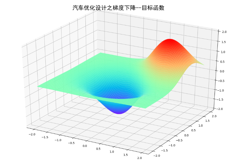
import numpy as np
from matplotlib import pyplot as plt
from mpl_toolkits.mplot3d import  Axes3D
def plot_3d():
    fig = plt.figure(figsize=(12,8))
    ax = Axes3D(fig)
    x = np.arange(-2,2,0.05)
    y = np.arange(-2,2,0.05)
    ##对x,y数据执行网格化
    x,y = np.meshgrid(x,y)
    z1 = np.exp(-x**2-y**2)
    z2 = np.exp(-(x-1)**2-(y-1)**2)
    z = -(z1-z2)*2
    ax.plot_surface(x,y,z,    ##x,y,z二维矩阵(坐标矩阵xv,yv,zv)
                    rstride=1,##retride(row)指定行的跨度
                    cstride=1,##retride(column)指定列的跨度
                    cmap='rainbow')  ##设置颜色映射
    ##设置z轴范围
    ax.set_zlim(-2,2)
    ##设置标题
    plt.title('优化设计之梯度下降--目标函数',fontproperties = 'SimHei',fontsize = 20)
    plt.show()
    ax.plot_surface()
plot_3d()
def plot_axes3d_wireframe():
    fig = plt.figure(figsize=(12,8))
    ax = Axes3D(fig)
    x = np.arange(-2,2,0.05)
    y = np.arange(-2,2,0.05)
    ##对x,y数据执行网格化
    x,y = np.meshgrid(x,y)
    z1 = np.exp(-x**2-y**2)
    z2 = np.exp(-(x-1)**2-(y-1)**2)
    z = -(z1-z2)*2
    ax.plot_wireframe(x,y,z,    ##x,y,z二维矩阵(坐标矩阵xv,yv,zv)
                    rstride=1,##retride(row)指定行的跨度
                    cstride=1,##retride(column)指定列的跨度
                    cmap='rainbow')  ##设置颜色映射
    ##设置z轴范围
    ax.set_zlim(-2,2)
    ##设置标题
    plt.title('优化设计之梯度下降--目标函数',fontproperties = 'SimHei',fontsize = 20)
    plt.show()
plot_axes3d_wireframe()

###二维散点图
##二维散点图
'''
matplotlib.pyplot.scatter(x, y, s=None, c=None, marker=None, cmap=None, norm=None,
                          vmin=None, vmax=None, alpha=None, linewidths=None,
                          verts=None, edgecolors=None, hold=None, data=None,
                          **kwargs)

x,y 平面点位置
s控制节点大小
c对应颜色值,c=x使点的颜色根据点的x值变化
cmap:颜色映射
marker:控制节点形状
alpha:控制节点透明度
'''

import numpy as np
import matplotlib.pyplot as plt

##二维散点图
fig = plt.figure()
x = np.arange(100)
y = np.random.randn(100)
plt.scatter(x,y,c='b')
plt.scatter(x+4,y,c='b',alpha=0.5)
plt.show()
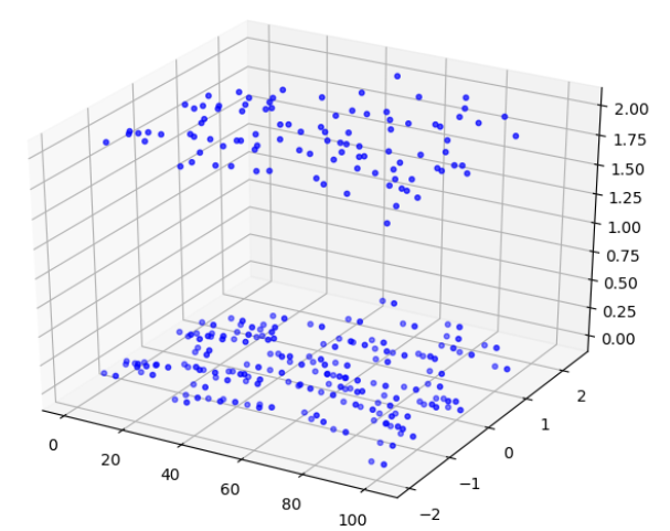
##三维散点图
'''
p3d.Axes3D.scatter( xs, ys, zs=0, zdir=’z’, s=20, c=None, depthshade=True,
                   *args, **kwargs )

p3d.Axes3D.scatter3D( xs, ys, zs=0, zdir=’z’, s=20, c=None, depthshade=True,
                   *args, **kwargs)
xs,ys 代表点x,y轴坐标
zs代表z轴坐标:第一种,标量z=0  在空间平面z=0画图,第二种z与xs,yx同样shape的数组
'''
import numpy as np
import matplotlib.pyplot as plt
from mpl_toolkits.mplot3d import Axes3D


fig = plt.figure()
ax  = Axes3D(fig)
x = np.arange(100)
y = np.random.randn(100)
ax.scatter(x,y,c='b',s=10,alpha=0.5)  ##默认z=0平面
ax.scatter(x+4,y,c='b',s=10,alpha=0.7)
ax.scatter(x+4,y,2,c='b',s=10,alpha=0.7)  ##指定z=2平面
plt.show()
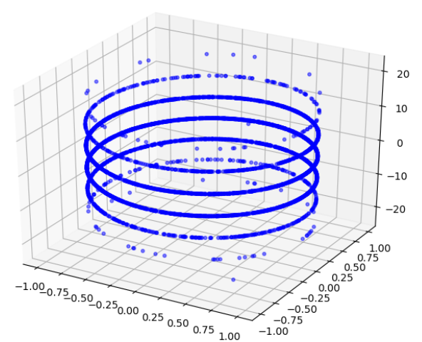
import numpy as np
import matplotlib.pyplot as plt
from mpl_toolkits.mplot3d import Axes3D

fig = plt.figure()
ax  = Axes3D(fig)
z = 6*np.random.randn(5000)
x = np.sin(z)
y = np.cos(z)
ax.scatter(x,y,z,c='b',s=10,alpha=0.5)
plt.show()
'''二维梯度下降法'''
def func_2d_single(x,y):
    '''
    目标函数传入x,y
    :param x,y: 自变量,一维向量
    :return: 因变量,标量
    '''
    z1 = np.exp(-x**2-y**2)
    z2 = np.exp(-(x-1)**2-(y-1)**2)
    z = -(z1-2*z2)*0.5
    return z

def func_2d(xy):
    '''
    目标函数传入xy组成的数组,如[x1,y1]
    :param xy: 自变量,二维向量  (x,y)
    :return: 因变量,标量
    '''
    z1 = np.exp(-xy[0]**2-xy[1]**2)
    z2 = np.exp(-(xy[0]-1)**2-(xy[1]-1)**2)
    z = -(z1-2*z2)*0.5
    return z
def grad_2d(xy):
    '''
    目标函数的梯度
    :param xy: 自变量,二维向量
    :return: 因变量,二维向量  (分别求偏导数,组成数组返回)
    '''
    grad_x = 2*xy[0]*(np.exp(-(xy[0]**2+xy[1]**2)))
    grad_y = 2*xy[1]*(np.exp(-(xy[0]**2+xy[1]**2)))
    return np.array([grad_x,grad_y])
def gradient_descent_2d(grad, cur_xy=np.array([1, 1]), learning_rate=0.001, precision=0.001, max_iters=100000000):
    '''
    二维目标函数的梯度下降法
    :param grad: 目标函数的梯度
    :param cur_xy: 当前的x和y值
    :param learning_rate: 学习率
    :param precision: 收敛精度
    :param max_iters: 最大迭代次数
    :return: 返回极小值
    '''
    print(f"{cur_xy} 作为初始值开始的迭代......")
    x_cur_list = []
    y_cur_list = []
    for i in tqdm(range(max_iters)):
        grad_cur = grad(cur_xy)
        ##创建两个列表,用于接收变化的x,y
        x_cur_list.append(cur_xy[0])
        y_cur_list.append(cur_xy[1])
        if np.linalg.norm(grad_cur,ord=2)<precision:  ##求范数,ord=2 平方和开根
            break    ###当梯度接近于0时,视为收敛
        cur_xy = cur_xy-grad_cur*learning_rate
        x_cur_list.append(cur_xy[0])
        y_cur_list.append(cur_xy[1])
        print('第%s次迭代:x,y = %s'%(i,cur_xy))
    print('极小值 x,y = %s '%cur_xy)
    return (x_cur_list,y_cur_list)
if __name__=="__main__":
    current_xy_list = gradient_descent_2d(grad_2d)
    fig = plt.figure(figsize=(12,8))
    ax = Axes3D(fig)
    a = np.array(current_xy_list[0])
    b = np.array(current_xy_list[1])
    c = func_2d_single(a,b)
    ax.scatter(a,b,c,c='Black',s=10,alpha=1,marker='o')
    x = np.arange(-2,2,0.05)
    y = np.arange(-2,2,0.05)
    ##对x,y数据执行网格化
    x,y = np.meshgrid(x,y)
    z = func_2d_single(x,y)
    ax.plot_surface(x,y,z,
                    rstride=1,##retride(row)指定行的跨度
                    cstride=1,##retride(column)指定列的跨度
                    cmap='rainbow',
                    alpha=0.3
                    )  ##设置颜色映射
    # ax.plot_wireframe(x,y,z,)
    ##设置z轴范围
    ax.set_zlim(-2,2)
    ##设置标题
    plt.title('汽车优化设计之梯度下降--二元函数',fontproperties = 'SimHei',fontsize = 20)
    plt.xlabel('x',fontproperties = 'SimHei',fontsize = 20)
    plt.ylabel('y', fontproperties='SimHei', fontsize=20)
    plt.show()
