Preprocessing data of sklearn

Preprocessing data

https://scikit-learn.org/stable/modules/preprocessing.html

数据预处理提供工具函数和变换器类，将转换特征向量成为更加适合下游模型的数据表示。

一般学习算法都会从数据标准化中受益。如果异常值存在于数据中，那么健壮的伸缩器和变换器是更加的合适。

几个相关概念：伸缩器（scaler）变换器（transformer）范数器（normalizer）

The sklearn.preprocessing package provides several common utility functions and transformer classes to change raw feature vectors into a representation that is more suitable for the downstream estimators.

In general, learning algorithms benefit from standardization of the data set. If some outliers are present in the set, robust scalers or transformers are more appropriate. The behaviors of the different scalers, transformers, and normalizers on a dataset containing marginal outliers is highlighted in Compare the effect of different scalers on data with outliers.

为什么叫数据预处理？

之所以叫preprocess，是因为这个阶段处理的数据还是属于pipeline中的最初的阶段，后续还有对数据的处理。

大部分工作在数据清洗和数据变换的范畴，在后续阶段存在特征提取和特征选择等工作，后续的工作是在本阶段数据之后进行的。

特征提取和特征选择对应数据规约。

https://zhuanlan.zhihu.com/p/89903181

根据自己的经验，总结了一下使用过的数据预处理的方法和小技巧。在进行数据分析的时候，工作量最大也最复杂的地方就是对数据进行预处理，一般分为四个步骤：数据清理、数据集成、数据变换、数据归约。

一、数据清理（缺失值、异常值、无关值、噪音、重复值）

二、数据集成

数据集成就是为了将不同数据源的数据整合导一个数据库中

数据变换和数据规约

个人觉得数据变换和数据规约其实等同于特征工程所要做的事，这里简单介绍下。
数据变换就是对数据做归一化，标准化等处理，例如不同的属性的值的量纲或者取值范围相差过大。
数据规约则是对减少过多的属性（维度、特征）对预测的模型的影响，常用方法：合并属性，主成成分分析（PCA），逐步向前（向后删除）、低方差特征过滤、one-hot编码等。

Standardization, or mean removal and variance scaling -- 标准化

将数据去均值按照方差进行伸缩，转换后的数据近似标准正太分布，很多机器学习算法需要这种类型的数据。

Standardization of datasets is a common requirement for many machine learning estimators implemented in scikit-learn; they might behave badly if the individual features do not more or less look like standard normally distributed data: Gaussian with zero mean and unit variance.

In practice we often ignore the shape of the distribution and just transform the data to center it by removing the mean value of each feature, then scale it by dividing non-constant features by their standard deviation.

The preprocessing module provides the StandardScaler utility class, which is a quick and easy way to perform the following operation on an array-like dataset:

>>> from sklearn import preprocessing
>>> import numpy as np
>>> X_train = np.array([[ 1., -1.,  2.],
...                     [ 2.,  0.,  0.],
...                     [ 0.,  1., -1.]])
>>> scaler = preprocessing.StandardScaler().fit(X_train)
>>> scaler
StandardScaler()

>>> scaler.mean_
array([1. ..., 0. ..., 0.33...])

>>> scaler.scale_
array([0.81..., 0.81..., 1.24...])

>>> X_scaled = scaler.transform(X_train)
>>> X_scaled
array([[ 0.  ..., -1.22...,  1.33...],
       [ 1.22...,  0.  ..., -0.26...],
       [-1.22...,  1.22..., -1.06...]])

StandardScaler

https://scikit-learn.org/stable/modules/generated/sklearn.preprocessing.StandardScaler.html#sklearn.preprocessing.StandardScaler

Standardize features by removing the mean and scaling to unit variance

The standard score of a sample x is calculated as:

z = (x - u) / s

where u is the mean of the training samples or zero if with_mean=False, and s is the standard deviation of the training samples or one if with_std=False.

Centering and scaling happen independently on each feature by computing the relevant statistics on the samples in the training set. Mean and standard deviation are then stored to be used on later data using transform.

Standardization of a dataset is a common requirement for many machine learning estimators: they might behave badly if the individual features do not more or less look like standard normally distributed data (e.g. Gaussian with 0 mean and unit variance).

>>> from sklearn.preprocessing import StandardScaler
>>> data = [[0, 0], [0, 0], [1, 1], [1, 1]]
>>> scaler = StandardScaler()
>>> print(scaler.fit(data))
StandardScaler()
>>> print(scaler.mean_)
[0.5 0.5]
>>> print(scaler.transform(data))
[[-1. -1.]
 [-1. -1.]
 [ 1.  1.]
 [ 1.  1.]]
>>> print(scaler.transform([[2, 2]]))
[[3. 3.]]

Scaling features to a range

另外标准化方法，将特征伸缩到规定的范围。

An alternative standardization is scaling features to lie between a given minimum and maximum value, often between zero and one, or so that the maximum absolute value of each feature is scaled to unit size. This can be achieved using MinMaxScaler or MaxAbsScaler, respectively.

The motivation to use this scaling include robustness to very small standard deviations of features and preserving zero entries in sparse data.

Here is an example to scale a toy data matrix to the [0, 1] range:

>>> X_train = np.array([[ 1., -1.,  2.],
...                     [ 2.,  0.,  0.],
...                     [ 0.,  1., -1.]])
...
>>> min_max_scaler = preprocessing.MinMaxScaler()
>>> X_train_minmax = min_max_scaler.fit_transform(X_train)
>>> X_train_minmax
array([[0.5       , 0.        , 1.        ],
       [1.        , 0.5       , 0.33333333],
       [0.        , 1.        , 0.        ]])

上面变换是按照最大值和最小值作为基准进行变换，变换范围为 [0, 1], 实际上有如下含义

If MinMaxScaler is given an explicit feature_range=(min, max) the full formula is:
X_std = (X - X.min(axis=0)) / (X.max(axis=0) - X.min(axis=0))

X_scaled = X_std * (max - min) + min

还有一种是按照最大的绝对值作为变换基准，变换后的范围是 [-1, 1]

MaxAbsScaler works in a very similar fashion, but scales in a way that the training data lies within the range [-1, 1] by dividing through the largest maximum value in each feature. It is meant for data that is already centered at zero or sparse data.

Here is how to use the toy data from the previous example with this scaler:

>>> X_train = np.array([[ 1., -1.,  2.],
...                     [ 2.,  0.,  0.],
...                     [ 0.,  1., -1.]])
...
>>> max_abs_scaler = preprocessing.MaxAbsScaler()
>>> X_train_maxabs = max_abs_scaler.fit_transform(X_train)
>>> X_train_maxabs
array([[ 0.5, -1. ,  1. ],
       [ 1. ,  0. ,  0. ],
       [ 0. ,  1. , -0.5]])
>>> X_test = np.array([[ -3., -1.,  4.]])
>>> X_test_maxabs = max_abs_scaler.transform(X_test)
>>> X_test_maxabs
array([[-1.5, -1. ,  2. ]])
>>> max_abs_scaler.scale_
array([2.,  1.,  2.])

MinMaxScaler

https://scikit-learn.org/stable/modules/generated/sklearn.preprocessing.MinMaxScaler.html#sklearn.preprocessing.MinMaxScaler

每个样本值都除以数据范围长度。

Transform features by scaling each feature to a given range.

This estimator scales and translates each feature individually such that it is in the given range on the training set, e.g. between zero and one.

The transformation is given by:
X_std = (X - X.min(axis=0)) / (X.max(axis=0) - X.min(axis=0))
X_scaled = X_std * (max - min) + min
where min, max = feature_range.

This transformation is often used as an alternative to zero mean, unit variance scaling.

>>> from sklearn.preprocessing import MinMaxScaler
>>> data = [[-1, 2], [-0.5, 6], [0, 10], [1, 18]]
>>> scaler = MinMaxScaler()
>>> print(scaler.fit(data))
MinMaxScaler()
>>> print(scaler.data_max_)
[ 1. 18.]
>>> print(scaler.transform(data))
[[0.   0.  ]
 [0.25 0.25]
 [0.5  0.5 ]
 [1.   1.  ]]
>>> print(scaler.transform([[2, 2]]))
[[1.5 0. ]]

MaxAbsScaler

https://scikit-learn.org/stable/modules/generated/sklearn.preprocessing.MaxAbsScaler.html#sklearn.preprocessing.MaxAbsScaler

每个数据样本都除以所有样本值的最大绝对值。

Scale each feature by its maximum absolute value.

This estimator scales and translates each feature individually such that the maximal absolute value of each feature in the training set will be 1.0. It does not shift/center the data, and thus does not destroy any sparsity.

This scaler can also be applied to sparse CSR or CSC matrices.

>>> from sklearn.preprocessing import MaxAbsScaler
>>> X = [[ 1., -1.,  2.],
...      [ 2.,  0.,  0.],
...      [ 0.,  1., -1.]]
>>> transformer = MaxAbsScaler().fit(X)
>>> transformer
MaxAbsScaler()
>>> transformer.transform(X)
array([[ 0.5, -1. ,  1. ],
       [ 1. ,  0. ,  0. ],
       [ 0. ,  1. , -0.5]])

Scaling sparse data

对于稀疏数据，中心化往往会破坏稀疏数据的特性，导致内存急剧增加。

其中 MaxAbsScaler 不会破坏数据稀疏性。但是如果特征在不同的尺度上，做伸缩是正确的，不用考虑稀疏性。

Centering sparse data would destroy the sparseness structure in the data, and thus rarely is a sensible thing to do. However, it can make sense to scale sparse inputs, especially if features are on different scales.

MaxAbsScaler was specifically designed for scaling sparse data, and is the recommended way to go about this. However, StandardScaler can accept scipy.sparse matrices as input, as long as with_mean=False is explicitly passed to the constructor. Otherwise a ValueError will be raised as silently centering would break the sparsity and would often crash the execution by allocating excessive amounts of memory unintentionally. RobustScaler cannot be fitted to sparse inputs, but you can use the transform method on sparse inputs.

Scaling data with outliers

对于异常数据，中心化和方差化是不能很好处理的。这些情况，可以使用 RobustScaler 。

If your data contains many outliers, scaling using the mean and variance of the data is likely to not work very well. In these cases, you can use RobustScaler as a drop-in replacement instead. It uses more robust estimates for the center and range of your data.

RobustScaler

https://scikit-learn.org/stable/modules/generated/sklearn.preprocessing.RobustScaler.html#sklearn.preprocessing.RobustScaler

使用统计的方法来伸缩特征，是健壮的对于异常点。

这里含义是，排除异常部分，在大多数的数据中寻找中心和方差。

Scale features using statistics that are robust to outliers.

This Scaler removes the median and scales the data according to the quantile range (defaults to IQR: Interquartile Range). The IQR is the range between the 1st quartile (25th quantile) and the 3rd quartile (75th quantile).

Centering and scaling happen independently on each feature by computing the relevant statistics on the samples in the training set. Median and interquartile range are then stored to be used on later data using the transform method.

Standardization of a dataset is a common requirement for many machine learning estimators. Typically this is done by removing the mean and scaling to unit variance. However, outliers can often influence the sample mean / variance in a negative way. In such cases, the median and the interquartile range often give better results.

>>> from sklearn.preprocessing import RobustScaler
>>> X = [[ 1., -2.,  2.],
...      [ -2.,  1.,  3.],
...      [ 4.,  1., -2.]]
>>> transformer = RobustScaler().fit(X)
>>> transformer
RobustScaler()
>>> transformer.transform(X)
array([[ 0. , -2. ,  0. ],
       [-1. ,  0. ,  0.4],
       [ 1. ,  0. , -1.6]])

Non-linear transformation

前面的变化都是线性变换，它们不改变数据的相对结构。

这里引入两种变换，来处理非线性数据：分位数变换和幂变换。这两种变化都能保证数据的单调性。幂变换将数据转化为近高斯分布。

Two types of transformations are available: quantile transforms and power transforms. Both quantile and power transforms are based on monotonic transformations of the features and thus preserve the rank of the values along each feature.

Power transforms are a family of parametric transformations that aim to map data from any distribution to as close to a Gaussian distribution.

Mapping to a Uniform distribution

均匀分布变换。

QuantileTransformer provides a non-parametric transformation to map the data to a uniform distribution with values between 0 and 1:

>>> from sklearn.datasets import load_iris
>>> from sklearn.model_selection import train_test_split
>>> X, y = load_iris(return_X_y=True)
>>> X_train, X_test, y_train, y_test = train_test_split(X, y, random_state=0)
>>> quantile_transformer = preprocessing.QuantileTransformer(random_state=0)
>>> X_train_trans = quantile_transformer.fit_transform(X_train)
>>> X_test_trans = quantile_transformer.transform(X_test)
>>> np.percentile(X_train[:, 0], [0, 25, 50, 75, 100]) 
array([ 4.3,  5.1,  5.8,  6.5,  7.9])

QuantileTransformer

https://scikit-learn.org/stable/modules/generated/sklearn.preprocessing.QuantileTransformer.html#sklearn.preprocessing.QuantileTransformer

Transform features using quantiles information.

This method transforms the features to follow a uniform or a normal distribution. Therefore, for a given feature, this transformation tends to spread out the most frequent values. It also reduces the impact of (marginal) outliers: this is therefore a robust preprocessing scheme.

The transformation is applied on each feature independently. First an estimate of the cumulative distribution function of a feature is used to map the original values to a uniform distribution. The obtained values are then mapped to the desired output distribution using the associated quantile function. Features values of new/unseen data that fall below or above the fitted range will be mapped to the bounds of the output distribution. Note that this transform is non-linear. It may distort linear correlations between variables measured at the same scale but renders variables measured at different scales more directly comparable.

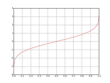
正太分布转换为均匀分布。

 

import numpy as np
from sklearn.preprocessing import QuantileTransformer
rng = np.random.RandomState(0)
X = np.sort(rng.normal(loc=0.5, scale=0.25, size=(25, 1)), axis=0)
qt = QuantileTransformer(n_quantiles=10, random_state=0)
qt.fit_transform(X)

array([[0.        ],
       [0.09871873],
       [0.10643612],
       [0.11754671],
       [0.21017437],
       [0.21945445],
       [0.23498666],
       [0.32443642],
       [0.33333333],
       [0.41360794],
       [0.42339464],
       [0.46257841],
       [0.47112236],
       [0.49834237],
       [0.59986536],
       [0.63390302],
       [0.66666667],
       [0.68873101],
       [0.69611125],
       [0.81280699],
       [0.82160354],
       [0.88126439],
       [0.90516028],
       [0.99319435],
       [1.        ]])

Quantile function

https://en.wikipedia.org/wiki/Quantile_function

分位数函数是关于随机变量的概率分布，指定一个随机变量的值，变量小于等于此值的概率等于给定的概率。类似现在考核上的强制分布，参考能力，将考核分为10个等级。

In probability and statistics, the quantile function, associated with a probability distribution of a random variable, specifies the value of the random variable such that the probability of the variable being less than or equal to that value equals the given probability. It is also called the percent-point function or inverse cumulative distribution function.

Mapping to a Gaussian distribution

映射任何数据分布到高斯分布。

In many modeling scenarios, normality of the features in a dataset is desirable. Power transforms are a family of parametric, monotonic transformations that aim to map data from any distribution to as close to a Gaussian distribution as possible in order to stabilize variance and minimize skewness.

PowerTransformer currently provides two such power transformations, the Yeo-Johnson transform and the Box-Cox transform.

>>> pt = preprocessing.PowerTransformer(method='box-cox', standardize=False)
>>> X_lognormal = np.random.RandomState(616).lognormal(size=(3, 3))
>>> X_lognormal
array([[1.28..., 1.18..., 0.84...],
       [0.94..., 1.60..., 0.38...],
       [1.35..., 0.21..., 1.09...]])
>>> pt.fit_transform(X_lognormal)
array([[ 0.49...,  0.17..., -0.15...],
       [-0.05...,  0.58..., -0.57...],
       [ 0.69..., -0.84...,  0.10...]])

PowerTransformer

https://scikit-learn.org/stable/modules/generated/sklearn.preprocessing.PowerTransformer.html#sklearn.preprocessing.PowerTransformer

Apply a power transform featurewise to make data more Gaussian-like.

Power transforms are a family of parametric, monotonic transformations that are applied to make data more Gaussian-like. This is useful for modeling issues related to heteroscedasticity (non-constant variance), or other situations where normality is desired.

Currently, PowerTransformer supports the Box-Cox transform and the Yeo-Johnson transform. The optimal parameter for stabilizing variance and minimizing skewness is estimated through maximum likelihood.

Box-Cox requires input data to be strictly positive, while Yeo-Johnson supports both positive or negative data.

By default, zero-mean, unit-variance normalization is applied to the transformed data.

>>> import numpy as np
>>> from sklearn.preprocessing import PowerTransformer
>>> pt = PowerTransformer()
>>> data = [[1, 2], [3, 2], [4, 5]]
>>> print(pt.fit(data))
PowerTransformer()
>>> print(pt.lambdas_)
[ 1.386... -3.100...]
>>> print(pt.transform(data))
[[-1.316... -0.707...]
 [ 0.209... -0.707...]
 [ 1.106...  1.414...]]

Normalization

范数化通过伸缩样本数据，将所有样本包含在单位范数空间。如果后续需要做点积计算，或者相似性计算，此变换是必要的。

范数有 l1, l2, or max。

Normalization is the process of scaling individual samples to have unit norm. This process can be useful if you plan to use a quadratic form such as the dot-product or any other kernel to quantify the similarity of any pair of samples.

This assumption is the base of the Vector Space Model often used in text classification and clustering contexts.

The function normalize provides a quick and easy way to perform this operation on a single array-like dataset, either using the l1, l2, or max norms:

>>> X = [[ 1., -1.,  2.],
...      [ 2.,  0.,  0.],
...      [ 0.,  1., -1.]]
>>> X_normalized = preprocessing.normalize(X, norm='l2')

>>> X_normalized
array([[ 0.40..., -0.40...,  0.81...],
       [ 1.  ...,  0.  ...,  0.  ...],
       [ 0.  ...,  0.70..., -0.70...]])

Normalizer

https://scikit-learn.org/stable/modules/generated/sklearn.preprocessing.Normalizer.html#sklearn.preprocessing.Normalizer

范数化样本到单位范数空间。在文本分类和聚类领域的常规操作。

Normalize samples individually to unit norm.

Each sample (i.e. each row of the data matrix) with at least one non zero component is rescaled independently of other samples so that its norm (l1, l2 or inf) equals one.

This transformer is able to work both with dense numpy arrays and scipy.sparse matrix (use CSR format if you want to avoid the burden of a copy / conversion).

Scaling inputs to unit norms is a common operation for text classification or clustering for instance. For instance the dot product of two l2-normalized TF-IDF vectors is the cosine similarity of the vectors and is the base similarity metric for the Vector Space Model commonly used by the Information Retrieval community.

>>> from sklearn.preprocessing import Normalizer
>>> X = [[4, 1, 2, 2],
...      [1, 3, 9, 3],
...      [5, 7, 5, 1]]
>>> transformer = Normalizer().fit(X)  # fit does nothing.
>>> transformer
Normalizer()
>>> transformer.transform(X)
array([[0.8, 0.2, 0.4, 0.4],
       [0.1, 0.3, 0.9, 0.3],
       [0.5, 0.7, 0.5, 0.1]])

Vector space model

https://en.wikipedia.org/wiki/Vector_space_model

向量空间模型，是文本文档的表示的代数模型。用于信息过滤获取索引相关性排名。

Vector space model or term vector model is an algebraic model for representing text documents (and any objects, in general) as vectors of identifiers (such as index terms). It is used in information filtering, information retrieval, indexing and relevancy rankings. Its first use was in the SMART Information Retrieval System.

Encoding categorical features

对于分类型特征，将类别名转换为整数。使用 OrdinalEncoder 序数编码器。

Often features are not given as continuous values but categorical. For example a person could have features ["male", "female"], ["from Europe", "from US", "from Asia"], ["uses Firefox", "uses Chrome", "uses Safari", "uses Internet Explorer"]. Such features can be efficiently coded as integers, for instance ["male", "from US", "uses Internet Explorer"] could be expressed as [0, 1, 3] while ["female", "from Asia", "uses Chrome"] would be [1, 2, 1].

To convert categorical features to such integer codes, we can use the OrdinalEncoder. This estimator transforms each categorical feature to one new feature of integers (0 to n_categories - 1):

>>> enc = preprocessing.OrdinalEncoder()
>>> X = [['male', 'from US', 'uses Safari'], ['female', 'from Europe', 'uses Firefox']]
>>> enc.fit(X)
OrdinalEncoder()
>>> enc.transform([['female', 'from US', 'uses Safari']])
array([[0., 1., 1.]])

序数编码器，转换后的数为整数，机器学习模型认为其为连续性特征，并且是有序的结构。这是不合适的。

另外一种替换方法是单热点变换 OneHotEncoder

Such integer representation can, however, not be used directly with all scikit-learn estimators, as these expect continuous input, and would interpret the categories as being ordered, which is often not desired (i.e. the set of browsers was ordered arbitrarily).

Another possibility to convert categorical features to features that can be used with scikit-learn estimators is to use a one-of-K, also known as one-hot or dummy encoding. This type of encoding can be obtained with the OneHotEncoder, which transforms each categorical feature with n_categories possible values into n_categories binary features, with one of them 1, and all others 0.

Continuing the example above:

>>> enc = preprocessing.OneHotEncoder()
>>> X = [['male', 'from US', 'uses Safari'], ['female', 'from Europe', 'uses Firefox']]
>>> enc.fit(X)
OneHotEncoder()
>>> enc.transform([['female', 'from US', 'uses Safari'],
...                ['male', 'from Europe', 'uses Safari']]).toarray()
array([[1., 0., 0., 1., 0., 1.],
       [0., 1., 1., 0., 0., 1.]])

OrdinalEncoder

https://scikit-learn.org/stable/modules/generated/sklearn.preprocessing.OrdinalEncoder.html#sklearn.preprocessing.OrdinalEncoder

Encode categorical features as an integer array.

The input to this transformer should be an array-like of integers or strings, denoting the values taken on by categorical (discrete) features. The features are converted to ordinal integers. This results in a single column of integers (0 to n_categories - 1) per feature.

>>> from sklearn.preprocessing import OrdinalEncoder
>>> enc = OrdinalEncoder()
>>> X = [['Male', 1], ['Female', 3], ['Female', 2]]
>>> enc.fit(X)
OrdinalEncoder()
>>> enc.categories_
[array(['Female', 'Male'], dtype=object), array([1, 2, 3], dtype=object)]
>>> enc.transform([['Female', 3], ['Male', 1]])
array([[0., 2.],
       [1., 0.]])

>>> enc.inverse_transform([[1, 0], [0, 1]])
array([['Male', 1],
       ['Female', 2]], dtype=object)

OneHotEncoder

https://scikit-learn.org/stable/modules/generated/sklearn.preprocessing.OneHotEncoder.html#sklearn.preprocessing.OneHotEncoder

Encode categorical features as a one-hot numeric array.

The input to this transformer should be an array-like of integers or strings, denoting the values taken on by categorical (discrete) features. The features are encoded using a one-hot (aka ‘one-of-K’ or ‘dummy’) encoding scheme. This creates a binary column for each category and returns a sparse matrix or dense array (depending on the sparse parameter)

By default, the encoder derives the categories based on the unique values in each feature. Alternatively, you can also specify the categories manually.

This encoding is needed for feeding categorical data to many scikit-learn estimators, notably linear models and SVMs with the standard kernels.

Note: a one-hot encoding of y labels should use a LabelBinarizer instead.

Given a dataset with two features, we let the encoder find the unique values per feature and transform the data to a binary one-hot encoding.

>>>
>>> from sklearn.preprocessing import OneHotEncoder

One can discard categories not seen during fit:

>>>
>>> enc = OneHotEncoder(handle_unknown='ignore')
>>> X = [['Male', 1], ['Female', 3], ['Female', 2]]
>>> enc.fit(X)
OneHotEncoder(handle_unknown='ignore')
>>> enc.categories_
[array(['Female', 'Male'], dtype=object), array([1, 2, 3], dtype=object)]
>>> enc.transform([['Female', 1], ['Male', 4]]).toarray()
array([[1., 0., 1., 0., 0.],
       [0., 1., 0., 0., 0.]])
>>> enc.inverse_transform([[0, 1, 1, 0, 0], [0, 0, 0, 1, 0]])
array([['Male', 1],
       [None, 2]], dtype=object)
>>> enc.get_feature_names(['gender', 'group'])
array(['gender_Female', 'gender_Male', 'group_1', 'group_2', 'group_3'],
  dtype=object)

One can always drop the first column for each feature:

>>>
>>> drop_enc = OneHotEncoder(drop='first').fit(X)
>>> drop_enc.categories_
[array(['Female', 'Male'], dtype=object), array([1, 2, 3], dtype=object)]
>>> drop_enc.transform([['Female', 1], ['Male', 2]]).toarray()
array([[0., 0., 0.],
       [1., 1., 0.]])

Or drop a column for feature only having 2 categories:

>>>
>>> drop_binary_enc = OneHotEncoder(drop='if_binary').fit(X)
>>> drop_binary_enc.transform([['Female', 1], ['Male', 2]]).toarray()
array([[0., 1., 0., 0.],
       [1., 0., 1., 0.]])

Discretization

离散化也是量化。将连续的特征转变为离散的值。

Discretization (otherwise known as quantization or binning) provides a way to partition continuous features into discrete values. Certain datasets with continuous features may benefit from discretization, because discretization can transform the dataset of continuous attributes to one with only nominal attributes.

One-hot encoded discretized features can make a model more expressive, while maintaining interpretability. For instance, pre-processing with a discretizer can introduce nonlinearity to linear models.

Discretization of continuous features

https://en.wikipedia.org/wiki/Discretization_of_continuous_features

一些算法是基于离散化数据

In statistics and machine learning, discretization refers to the process of converting or partitioning continuous attributes, features or variables to discretized or nominal attributes/features/variables/intervals. This can be useful when creating probability mass functions – formally, in density estimation. It is a form of discretization in general and also of binning, as in making a histogram. Whenever continuous data is discretized, there is always some amount of discretization error. The goal is to reduce the amount to a level considered negligible for the modeling purposes at hand.

Typically data is discretized into partitions of K equal lengths/width (equal intervals) or K% of the total data (equal frequencies).^[1]

Mechanisms for discretizing continuous data include Fayyad & Irani's MDL method,^[2] which uses mutual information to recursively define the best bins, CAIM, CACC, Ameva, and many others^[3]

Many machine learning algorithms are known to produce better models by discretizing continuous attributes.^[4]

K-bins discretization

KBinsDiscretizer discretizes features into k bins:

X = np.array([[ -3., 5., 15 ],
              [  0., 6., 14 ],
              [  6., 3., 11 ]])
est = preprocessing.KBinsDiscretizer(n_bins=[3, 2, 2], encode='ordinal').fit(X)

>>> est.transform(X)                      
array([[ 0., 1., 1.],
       [ 1., 1., 1.],
       [ 2., 0., 0.]])

KBinsDiscretizer

https://scikit-learn.org/stable/modules/generated/sklearn.preprocessing.KBinsDiscretizer.html#sklearn.preprocessing.KBinsDiscretizer

Bin continuous data into intervals.

>>> X = [[-2, 1, -4,   -1],
...      [-1, 2, -3, -0.5],
...      [ 0, 3, -2,  0.5],
...      [ 1, 4, -1,    2]]
>>> est = KBinsDiscretizer(n_bins=3, encode='ordinal', strategy='uniform')
>>> est.fit(X)
KBinsDiscretizer(...)
>>> Xt = est.transform(X)
>>> Xt  
array([[ 0., 0., 0., 0.],
       [ 1., 1., 1., 0.],
       [ 2., 2., 2., 1.],
       [ 2., 2., 2., 2.]])

Feature binarization

特征二值化，将数值类型特征转换为布尔值，给出阈值。应用于贝努力分布。

Feature binarization is the process of thresholding numerical features to get boolean values. This can be useful for downstream probabilistic estimators that make assumption that the input data is distributed according to a multi-variate Bernoulli distribution. For instance, this is the case for the BernoulliRBM.

It is also common among the text processing community to use binary feature values (probably to simplify the probabilistic reasoning) even if normalized counts (a.k.a. term frequencies) or TF-IDF valued features often perform slightly better in practice.

As for the Normalizer, the utility class Binarizer is meant to be used in the early stages of Pipeline. The fit method does nothing as each sample is treated independently of others:

>>> X = [[ 1., -1.,  2.],
...      [ 2.,  0.,  0.],
...      [ 0.,  1., -1.]]

>>> binarizer = preprocessing.Binarizer().fit(X)  # fit does nothing
>>> binarizer
Binarizer()

>>> binarizer.transform(X)
array([[1., 0., 1.],
       [1., 0., 0.],
       [0., 1., 0.]])

Bernoulli distribution

https://en.wikipedia.org/wiki/Bernoulli_distribution

二项分布。

The Bernoulli distribution is a special case of the binomial distribution where a single trial is conducted (so n would be 1 for such a binomial distribution). It is also a special case of the two-point distribution, for which the possible outcomes need not be 0 and 1.

$p$

$p$

$p$

$p$

Binarizer

https://scikit-learn.org/stable/modules/generated/sklearn.preprocessing.Binarizer.html#sklearn.preprocessing.Binarizer

Binarize data (set feature values to 0 or 1) according to a threshold.

Values greater than the threshold map to 1, while values less than or equal to the threshold map to 0. With the default threshold of 0, only positive values map to 1.

Binarization is a common operation on text count data where the analyst can decide to only consider the presence or absence of a feature rather than a quantified number of occurrences for instance.

It can also be used as a pre-processing step for estimators that consider boolean random variables (e.g. modelled using the Bernoulli distribution in a Bayesian setting).

Imputation of missing values

https://scikit-learn.org/stable/modules/impute.html#impute

不能简单地删除样本，对于样本比较少的情况，也会损失其它有用信息。

For various reasons, many real world datasets contain missing values, often encoded as blanks, NaNs or other placeholders. Such datasets however are incompatible with scikit-learn estimators which assume that all values in an array are numerical, and that all have and hold meaning. A basic strategy to use incomplete datasets is to discard entire rows and/or columns containing missing values. However, this comes at the price of losing data which may be valuable (even though incomplete). A better strategy is to impute the missing values, i.e., to infer them from the known part of the data. See the Glossary of Common Terms and API Elements entry on imputation.

Univariate feature imputation

使用本特征的值的特征，例如均值和中位数，来填补。

The SimpleImputer class provides basic strategies for imputing missing values. Missing values can be imputed with a provided constant value, or using the statistics (mean, median or most frequent) of each column in which the missing values are located. This class also allows for different missing values encodings.

The following snippet demonstrates how to replace missing values, encoded as np.nan, using the mean value of the columns (axis 0) that contain the missing values:

>>> import numpy as np
>>> from sklearn.impute import SimpleImputer
>>> imp = SimpleImputer(missing_values=np.nan, strategy='mean')
>>> imp.fit([[1, 2], [np.nan, 3], [7, 6]])
SimpleImputer()
>>> X = [[np.nan, 2], [6, np.nan], [7, 6]]
>>> print(imp.transform(X))
[[4.          2.        ]
 [6.          3.666...]
 [7.          6.        ]]

Multivariate feature imputation

建立回归预测缺失值，使用其它特征值，来预测确实值。

A more sophisticated approach is to use the IterativeImputer class, which models each feature with missing values as a function of other features, and uses that estimate for imputation. It does so in an iterated round-robin fashion: at each step, a feature column is designated as output y and the other feature columns are treated as inputs X. A regressor is fit on (X, y) for known y. Then, the regressor is used to predict the missing values of y. This is done for each feature in an iterative fashion, and then is repeated for max_iter imputation rounds. The results of the final imputation round are returned.

>>> import numpy as np
>>> from sklearn.experimental import enable_iterative_imputer
>>> from sklearn.impute import IterativeImputer
>>> imp = IterativeImputer(max_iter=10, random_state=0)
>>> imp.fit([[1, 2], [3, 6], [4, 8], [np.nan, 3], [7, np.nan]])
IterativeImputer(random_state=0)
>>> X_test = [[np.nan, 2], [6, np.nan], [np.nan, 6]]
>>> # the model learns that the second feature is double the first
>>> print(np.round(imp.transform(X_test)))
[[ 1.  2.]
 [ 6. 12.]
 [ 3.  6.]]

Nearest neighbors imputation

使用K近邻思想来填补缺失值。

The KNNImputer class provides imputation for filling in missing values using the k-Nearest Neighbors approach. By default, a euclidean distance metric that supports missing values, nan_euclidean_distances, is used to find the nearest neighbors. Each missing feature is imputed using values from n_neighbors nearest neighbors that have a value for the feature. The feature of the neighbors are averaged uniformly or weighted by distance to each neighbor. If a sample has more than one feature missing, then the neighbors for that sample can be different depending on the particular feature being imputed. When the number of available neighbors is less than n_neighbors and there are no defined distances to the training set, the training set average for that feature is used during imputation. If there is at least one neighbor with a defined distance, the weighted or unweighted average of the remaining neighbors will be used during imputation. If a feature is always missing in training, it is removed during transform. For more information on the methodology, see ref. [OL2001].

The following snippet demonstrates how to replace missing values, encoded as np.nan, using the mean feature value of the two nearest neighbors of samples with missing values:

>>> import numpy as np
>>> from sklearn.impute import KNNImputer
>>> nan = np.nan
>>> X = [[1, 2, nan], [3, 4, 3], [nan, 6, 5], [8, 8, 7]]
>>> imputer = KNNImputer(n_neighbors=2, weights="uniform")
>>> imputer.fit_transform(X)
array([[1. , 2. , 4. ],
       [3. , 4. , 3. ],
       [5.5, 6. , 5. ],
       [8. , 8. , 7. ]])

Custom transformers

对于个性化变化，可以自己定义对数据的变换逻辑。

Often, you will want to convert an existing Python function into a transformer to assist in data cleaning or processing. You can implement a transformer from an arbitrary function with FunctionTransformer. For example, to build a transformer that applies a log transformation in a pipeline, do:

>>> import numpy as np
>>> from sklearn.preprocessing import FunctionTransformer
>>> transformer = FunctionTransformer(np.log1p, validate=True)
>>> X = np.array([[0, 1], [2, 3]])
>>> transformer.transform(X)
array([[0.        , 0.69314718],
       [1.09861229, 1.38629436]])

Compare the effect of different scalers on data with outliers

https://scikit-learn.org/stable/auto_examples/preprocessing/plot_all_scaling.html#maxabsscaler

对于异常值，伸缩器是线性变化，不同点是估计参数的方法，估计后的参数用于平移数据，和以中心点为中心伸缩数据。

QuantileTransformer 提供非线性信息，其中边际异常点和内部点之间的距离被萎缩了。

PowerTransformer提供非线性信息，其中数据被映射到正态分布上，来稳定化方差，极小化偏差。

范数化是涉及单个样本的变换，并不对正特特征分布的变化。

Feature 0 (median income in a block) and feature 5 (number of households) of the California Housing dataset have very different scales and contain some very large outliers. These two characteristics lead to difficulties to visualize the data and, more importantly, they can degrade the predictive performance of many machine learning algorithms. Unscaled data can also slow down or even prevent the convergence of many gradient-based estimators.

Indeed many estimators are designed with the assumption that each feature takes values close to zero or more importantly that all features vary on comparable scales. In particular, metric-based and gradient-based estimators often assume approximately standardized data (centered features with unit variances). A notable exception are decision tree-based estimators that are robust to arbitrary scaling of the data.

This example uses different scalers, transformers, and normalizers to bring the data within a pre-defined range.

Scalers are linear (or more precisely affine) transformers and differ from each other in the way they estimate the parameters used to shift and scale each feature.

QuantileTransformer provides non-linear transformations in which distances between marginal outliers and inliers are shrunk. PowerTransformer provides non-linear transformations in which data is mapped to a normal distribution to stabilize variance and minimize skewness.

Unlike the previous transformations, normalization refers to a per sample transformation instead of a per feature transformation.

Feature discretization

https://scikit-learn.org/stable/auto_examples/preprocessing/plot_discretization_classification.html#sphx-glr-auto-examples-preprocessing-plot-discretization-classification-py

对于线性不可分数据，使用线性模型，应用特征离散化，有助于提高性能。可以理解为，离散化为线性模型提供了更多的信息。

对于线性可分数据，使用线性模型，则不需要进行特征离散化。会破坏线性化提供的信息。

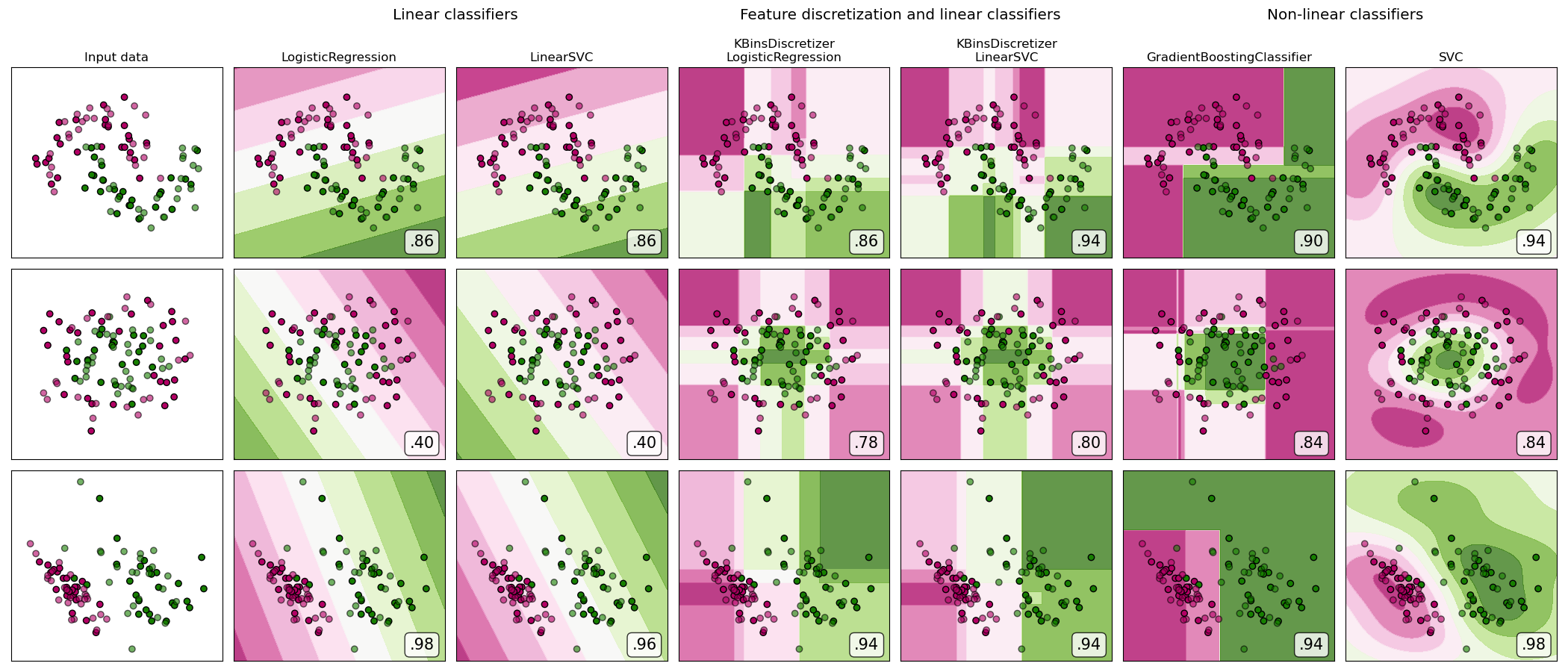
A demonstration of feature discretization on synthetic classification datasets. Feature discretization decomposes each feature into a set of bins, here equally distributed in width. The discrete values are then one-hot encoded, and given to a linear classifier. This preprocessing enables a non-linear behavior even though the classifier is linear.

On this example, the first two rows represent linearly non-separable datasets (moons and concentric circles) while the third is approximately linearly separable. On the two linearly non-separable datasets, feature discretization largely increases the performance of linear classifiers. On the linearly separable dataset, feature discretization decreases the performance of linear classifiers. Two non-linear classifiers are also shown for comparison.

This example should be taken with a grain of salt, as the intuition conveyed does not necessarily carry over to real datasets. Particularly in high-dimensional spaces, data can more easily be separated linearly. Moreover, using feature discretization and one-hot encoding increases the number of features, which easily lead to overfitting when the number of samples is small.

The plots show training points in solid colors and testing points semi-transparent. The lower right shows the classification accuracy on the test set.

Out:
dataset 0
---------
LogisticRegression: 0.86
LinearSVC: 0.86
KBinsDiscretizer + LogisticRegression: 0.86
KBinsDiscretizer + LinearSVC: 0.92
GradientBoostingClassifier: 0.90
SVC: 0.94

dataset 1
---------
LogisticRegression: 0.40
LinearSVC: 0.40
KBinsDiscretizer + LogisticRegression: 0.88
KBinsDiscretizer + LinearSVC: 0.86
GradientBoostingClassifier: 0.80
SVC: 0.84

dataset 2
---------
LogisticRegression: 0.98
LinearSVC: 0.98
KBinsDiscretizer + LogisticRegression: 0.94
KBinsDiscretizer + LinearSVC: 0.94
GradientBoostingClassifier: 0.88
SVC: 0.98

numpy.logspace

https://numpy.org/doc/stable/reference/generated/numpy.logspace.html#numpy.logspace

将一个等差数列，以常数递增的数列，变换为加速递增的数列。

一般引用语参数调优，例如学习速率。

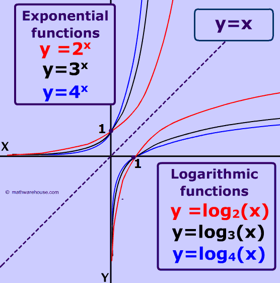
Return numbers spaced evenly on a log scale.

In linear space, the sequence starts at base ** start (base to the power of start) and ends with base ** stop (see endpoint below).

log函数是幂函数的对数函数。

Examples

>>>

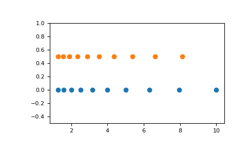
np.logspace(2.0, 3.0, num=4)
array([ 100.        ,  215.443469  ,  464.15888336, 1000.        ])

np.logspace(2.0, 3.0, num=4, endpoint=False)
array([100.        ,  177.827941  ,  316.22776602,  562.34132519])

np.logspace(2.0, 3.0, num=4, base=2.0)
array([4.        ,  5.0396842 ,  6.34960421,  8.        ])

Graphical illustration:

>>>

import matplotlib.pyplot as plt

N = 10

x1 = np.logspace(0.1, 1, N, endpoint=True)

x2 = np.logspace(0.1, 1, N, endpoint=False)

y = np.zeros(N)

plt.plot(x1, y, 'o')
[<matplotlib.lines.Line2D object at 0x...>]

plt.plot(x2, y + 0.5, 'o')
[<matplotlib.lines.Line2D object at 0x...>]

plt.ylim([-0.5, 1])
(-0.5, 1)

plt.show()

出处：http://www.cnblogs.com/lightsong/ 本文版权归作者和博客园共有,欢迎转载,但未经作者同意必须保留此段声明,且在文章页面明显位置给出原文连接。