目录
预创建的 Estimator (pre-made Estimator)
自定义 Estimator(custom Estimator)
TensorFlow是一个 可用于构建机器学习模型的平台。但其实它的用途范围要广泛得多。它是一种基于图表的通用计算框架, 可用来编写您能想出的任何东西。事实上,TensorFlow.org的API页面中提供了可在代码中使用的低级TensorFlow运算的完整列表。贡献者们还添加了多个可以让我们轻松地执行常见任务的高级框架。您将会最为频繁地使用TensorFlow Estimator API, 此API极大地简化了神经网络模型的构建过程。
1.工具包

图 1. TensorFlow 工具包层次结构。
我们建议您先从最高级 API 入手,让所有组件正常运作起来。如果您希望在某些特殊建模方面能够更加灵活一些,则可以降低一个级别。
TensorFlow
一个大型的分布式机器学习平台。该术语还指 TensorFlow 堆栈中的基本 API 层,该层支持对数据流图进行一般计算。
虽然 TensorFlow 主要应用于机器学习领域,但也可用于需要使用数据流图进行数值计算的非机器学习任务。
TensorFlow 由以下两个组件组成:
这两个组件类似于 Java 编译器和 JVM。正如 JVM 会实施在多个硬件平台(CPU 和 GPU)上一样,TensorFlow 也是如此。
张量 (Tensor)
TensorFlow 程序中的主要数据结构。
张量是 N 维(其中 N 可能非常大)数据结构,最常见的是标量、向量或矩阵。
张量的元素可以包含整数值、浮点值或字符串值。
图 (graph)
TensorFlow 中的一种计算规范。
图中的节点表示操作。边缘具有方向,表示将某项操作的结果(一个张量)作为一个操作数传递给另一项操作。
可以使用 TensorBoard 直观呈现图。
TensorBoard
一个信息中心,用于显示在执行一个或多个 TensorFlow 程序期间保存的摘要信息。
2.tf.estimator API
tf.estimator 与 scikit-learn API 兼容。
scikit-learn 是极其热门的 Python 开放源代码机器学习库,拥有超过 10 万名用户,其中包括许多 Google 员工。
概括而言,以下是在 tf.estimator 中实现的线性回归程序的格式:
import tensorflow as tf
# Set up a linear classifier.
classifier = tf.estimator.LinearClassifier()
# Train the model on some example data.
classifier.train(input_fn=train_input_fn, steps=2000)
# Use it to predict.
predictions = classifier.predict(input_fn=predict_input_fn)
Estimator
tf.Estimator类的一个实例,用于封装负责构建 TensorFlow 图并运行 TensorFlow 会话的逻辑。预创建的 Estimator (pre-made Estimator)
其他人已建好的 Estimator。
TensorFlow 提供了一些预创建的 Estimator,包括
DNNClassifier、DNNRegressor和LinearClassifier。自定义 Estimator(custom Estimator)
您可以按照这些说明(https://www.tensorflow.org/guide/custom_estimators)构建。
3.编程练习
1)Pandas 简介
作业上传到了github:https://github.com/hoshinotsuki/ML_google/blob/master/intro_to_pandas.ipynb
- 大致了解 pandas 库的
DataFrame和Series数据结构 - 存取和处理
DataFrame和Series中的数据 - 将 CSV 数据导入 pandas 库的
DataFrame - 对
DataFrame重建索引来随机打乱数据
pandas 是一种列存数据分析 API。有关更完整的参考,请访问 pandas 文档网站,其中包含丰富的文档和教程资源。
2)使用 TensorFlow 的起始步骤
此练习介绍了线性回归。
作业上传到了github:https://github.com/hoshinotsuki/ML_google/blob/master/first_steps_with_tensor_flow.ipynb
- 学习基本的 TensorFlow 概念
- 在 TensorFlow 中使用
LinearRegressor类并基于单个输入特征预测各城市街区的房屋价值中位数 - 使用均方根误差 (RMSE) 评估模型预测的准确率
- 通过调整模型的超参数提高模型准确率
tensorflow建模基本步骤
一、设置
1.加载库
from __future__ import print_function

import math

from IPython import display
from matplotlib import cm
from matplotlib import gridspec
from matplotlib import pyplot as plt
import numpy as np
import pandas as pd
from sklearn import metrics
import tensorflow as tf
from tensorflow.python.data import Dataset

tf.logging.set_verbosity(tf.logging.ERROR)
pd.options.display.max_rows = 10
pd.options.display.float_format = '{:.1f}'.format
bug 1:win10下用jupyter进入到tensorflow环境失败
解决:在anaconda navigator里install jupyter notebook。
ref:使用anaconda安装Tensorflow+在spyder和jupyter中启动Tensorflow
bug 2:ModuleNotFoundError: No module named '包名'
(env) > conda install 包名2.加载数据集
california_housing_dataframe = pd.read_csv("https://download.mlcc.google.com/mledu-datasets/california_housing_train.csv", sep=",")bug 3:数据下载慢,打不开
直接下到本地读取。ref:pandas.read_csv参数整理
california_housing_dataframe = pd.read_csv("D:/datas/california_housing_train.csv", sep=",") 3.随机化处理数据 ,调整目标的单位
california_housing_dataframecalifor  = california_housing_dataframe.reindex(np.random.permutation(california_housing_dataframe.index))
california_housing_dataframe["median_house_value"] /= 1000.0
california_housing_dataframe
二、检查数据
实用统计信息快速摘要:样本数、均值、标准偏差、最大值、最小值和各种分位数
california_housing_dataframe.describe()
三、构建第一个模型
3.定义特征、配置特征列
为了将训练数据导入 tensorflow , 要指定每个特征包含的数据类型,主要分为两类。
- 分类数据:文字
- 数值数据:数字(int或float)
特征列:表示特征的数据类型。只存储描述,不存储数据本身。
- 从dataframe中提取特征数据total_rooms。
- 用
numeric_column定义特征列,将特征数据指定为数值。是一个一维数组,是numeric_column的默认形状。
# Define the input feature: total_rooms.
my_feature = california_housing_dataframe[["total_rooms"]]
# Configure a numeric feature column for total_rooms.
feature_columns = [tf.feature_column.numeric_column("total_rooms")]
california_housing_dataframe[["total_rooms"]] 与california_housing_dataframe["total_rooms"]
california_housing_dataframe[["total_rooms"]] 是一个dataframe,传递给输入特征

california_housing_dataframe["total_rooms"]是一个一维数组
查看特征列存储内容:数据类型的描述。


4.定义目标
从dataframe中提取 目标median_house_value。
# Define the label.
targets = california_housing_dataframe["median_house_value"]
target也是一维数组

5.用LinearRegressor配置线性回归模型
使用 GradientDescentOptimizer(小批量随机梯度下降法 (SGD))训练该模型。learning_rate 控制梯度步长的大小。上期说了梯度步长=学习率*步长。语法:API.GradientDescentOptimizer(学习率)
# Use gradient descent as the optimizer for training the model.
my_optimizer=tf.train.GradientDescentOptimizer(learning_rate=0.0000001)
通过 clip_gradients_by_norm 将梯度裁剪应用到优化器。梯度裁剪可确保梯度大小在训练期间不会变得过大,梯度过大会导致梯度下降法失败。语法:API.clip_gradients_by_norm(优化器,梯度上限)
my_optimizer = tf.contrib.estimator.clip_gradients_by_norm(my_optimizer, 5.0)
梯度裁剪 (gradient clipping)
在应用梯度值之前先设置其上限。梯度裁剪有助于确保数值稳定性以及防止梯度爆炸【论文:L15 Exploding and Vanishing Gradients】。
用LinearRegressor配置线性回归模型 。语法:API.LinearRegressor(特征列,优化器)
# Configure the linear regression model with our feature columns and optimizer.
# Set a learning rate of 0.0000001 for Gradient Descent.
linear_regressor = tf.estimator.LinearRegressor(
    feature_columns=feature_columns,
    optimizer=my_optimizer
)
6.定义输入函数
让输入函数告诉 TensorFlow 如何对数据进行预处理,以及在模型训练期间如何批处理、随机处理和重复数据。
def my_input_fn(features, targets, batch_size=1, shuffle=True, num_epochs=None):
    """Trains a linear regression model of one feature.

    Args:
      features: pandas DataFrame of features
      targets: pandas DataFrame of targets
      batch_size: Size of batches to be passed to the model
      shuffle: True or False. Whether to shuffle the data.
      num_epochs: Number of epochs for which data should be repeated. None = repeat indefinitely
    Returns:
      Tuple of (features, labels) for next data batch
    """

    # Convert pandas data into a dict of np arrays.
    features = {key:np.array(value) for key,value in dict(features).items()}

    # Construct a dataset, and configure batching/repeating
    ds = Dataset.from_tensor_slices((features,targets)) # warning: 2GB limit
    ds = ds.batch(batch_size).repeat(num_epochs)

    # Shuffle the data, if specified
    if shuffle:
      ds = ds.shuffle(buffer_size=10000)

    # Return the next batch of data
    features, labels = ds.make_one_shot_iterator().get_next()
    return features, labels
输入函数和 Dataset API 的更详细的文档,请参阅 TensorFlow 编程人员指南。
- 将 Pandas 特征数据转换成 NumPy 数组字典
- 使用 TensorFlow Dataset API 根据我们的数据构建 Dataset 对象。
- 将dataset拆分成大小为
batch_size的多批数据,以按照指定周期数 (num_epochs) 进行重复。如果将默认值num_epochs=None传递到repeat(),输入数据会无限期重复。 - 如果
shuffle设置为True,则我们会对数据进行随机处理,以便数据在训练期间以随机方式传递到模型。buffer_size参数会指定shuffle将从中随机抽样的数据集的大小。 - 输入函数会为该数据集构建一个迭代器make_one_shot_iterator(),并向 LinearRegressor 返回下一批数据get_next()。
7.训练模型
在 linear_regressor 上调用 train() 来训练模型。语法:API.train(输入函数,步长)
将 my_input_fn 封装在 lambda 中,以便可以将 my_feature 和 target 作为参数传入(有关详情,请参阅此 TensorFlow 输入函数教程)
_ = linear_regressor.train(
    input_fn = lambda:my_input_fn(my_feature, targets),
    steps=100
)
8.评估模型
# Create an input function for predictions.
# Note: Since we're making just one prediction for each example, we don't need to repeat or shuffle the data here.
prediction_input_fn =lambda: my_input_fn(my_feature, targets, num_epochs=1, shuffle=False)
#<function __main__.<lambda>>

# Call predict() on the linear_regressor to make predictions.
predictions = linear_regressor.predict(input_fn=prediction_input_fn)
#<generator object predict at 0x7f640ef5ba00>

# Format predictions as a NumPy array, so we can calculate error metrics.
predictions = np.array([item['predictions'][0] for item in predictions])
#array([0.10574976, 0.18444955, 0.5131987 , ..., 0.16114962, 0.02299998, 0.11534974], dtype=float32)

# Print Mean Squared Error and Root Mean Squared Error.
mean_squared_error = metrics.mean_squared_error(predictions, targets)
root_mean_squared_error = math.sqrt(mean_squared_error)
print("Mean Squared Error (on training data): %0.3f" % mean_squared_error)
#Mean Squared Error (on training data): 56367.025
print("Root Mean Squared Error (on training data): %0.3f" % root_mean_squared_error)
#Root Mean Squared Error (on training data): 237.417
比较一下 RMSE 与目标最大值和最小值的差值
min_house_value = california_housing_dataframe["median_house_value"].min()
max_house_value = california_housing_dataframe["median_house_value"].max()
min_max_difference = max_house_value - min_house_value

print("Min. Median House Value: %0.3f" % min_house_value)
#Min. Median House Value: 14.999
print("Max. Median House Value: %0.3f" % max_house_value)
#Max. Median House Value: 500.001
print("Difference between Min. and Max.: %0.3f" % min_max_difference)
#Difference between Min. and Max.: 485.002
print("Root Mean Squared Error: %0.3f" % root_mean_squared_error)
#Root Mean Squared Error: 237.417
根据总体摘要统计信息,查看预测和目标的符合情况。
calibration_data = pd.DataFrame()
calibration_data["predictions"] = pd.Series(predictions)
calibration_data["targets"] = pd.Series(targets)
calibration_data.describe()
可视化
9.获取均匀分布的随机样本
sample = california_housing_dataframe.sample(n=300)10.根据模型的偏差项和特征权重绘制学到的线
# Get the min and max total_rooms values.
x_0 = sample["total_rooms"].min()
x_1 = sample["total_rooms"].max()

# Retrieve the final weight and bias generated during training.
weight = linear_regressor.get_variable_value('linear/linear_model/total_rooms/weights')[0]
bias = linear_regressor.get_variable_value('linear/linear_model/bias_weights')

# Get the predicted median_house_values for the min and max total_rooms values.
y_0 = weight * x_0 + bias
y_1 = weight * x_1 + bias

# Plot our regression line from (x_0, y_0) to (x_1, y_1).
plt.plot([x_0, x_1], [y_0, y_1], c='r')

# Label the graph axes.
plt.ylabel("median_house_value")
plt.xlabel("total_rooms")

# Plot a scatter plot from our data sample.
plt.scatter(sample["total_rooms"], sample["median_house_value"])

# Display graph.
plt.show()
四、调整模型超参数
def train_model(learning_rate, steps, batch_size, input_feature="total_rooms"):
  """Trains a linear regression model of one feature.

  Args:
    learning_rate: A `float`, the learning rate.
    steps: A non-zero `int`, the total number of training steps. A training step
      consists of a forward and backward pass using a single batch.
    batch_size: A non-zero `int`, the batch size.
    input_feature: A `string` specifying a column from `california_housing_dataframe`
      to use as input feature.
  """

  # 在 10 个等分的时间段内使用此函数,以便观察模型在每个时间段的改善情况。
  periods = 10
  steps_per_period = steps / periods

  # 1.定义特征
  my_feature = input_feature
  my_feature_data = california_housing_dataframe[[my_feature]]
  # 配置特征列
  feature_columns = [tf.feature_column.numeric_column(my_feature)]


  # 2.定义目标
  my_label = "median_house_value"
  targets = california_housing_dataframe[my_label]

  # 3.配置LinearRegressor
  # 优化器用SGD
  my_optimizer = tf.train.GradientDescentOptimizer(learning_rate=learning_rate)
  # 梯度裁剪
  my_optimizer = tf.contrib.estimator.clip_gradients_by_norm(my_optimizer, 5.0)
  # 创建一个线性回归对象
  linear_regressor = tf.estimator.LinearRegressor(
      feature_columns=feature_columns,
      optimizer=my_optimizer
  )

  # 4.定义输入函数
  training_input_fn = lambda:my_input_fn(my_feature_data, targets, batch_size=batch_size)
  prediction_input_fn = lambda: my_input_fn(my_feature_data, targets, num_epochs=1, shuffle=False)


  # Set up to plot the state of our model's line each period.
  plt.figure(figsize=(15, 6))
  plt.subplot(1, 2, 1)
  plt.title("Learned Line by Period")
  plt.ylabel(my_label)
  plt.xlabel(my_feature)
  sample = california_housing_dataframe.sample(n=300)
  plt.scatter(sample[my_feature], sample[my_label])
  colors = [cm.coolwarm(x) for x in np.linspace(-1, 1, periods)]

  # 5.训练模型
  #  Train the model, but do so inside a loop so that we can periodically assess loss metrics.对于每个时间段,我们都会计算训练损失并绘制相应图表。

  print("Training model...")
  print("RMSE (on training data):")
  root_mean_squared_errors = []
  for period in range (0, periods):

    # 训练模型Train the model, starting from the prior state.
    linear_regressor.train(
        input_fn=training_input_fn,
        steps=steps_per_period
    )

    # 预测Take a break and compute predictions.
    predictions = linear_regressor.predict(input_fn=prediction_input_fn)
    predictions = np.array([item['predictions'][0] for item in predictions])

    # 计算损失rmse
    root_mean_squared_error = math.sqrt(
        metrics.mean_squared_error(predictions, targets))

    # 打印当前损失
    print("  period %02d : %0.2f" % (period, root_mean_squared_error))

    # 将rmse记录到列表
    root_mean_squared_errors.append(root_mean_squared_error)

    # 跟踪这个过程中的权重和变量
    # Apply some math to ensure that the data and line are plotted neatly.
    y_extents = np.array([0, sample[my_label].max()])

    # 获取模型中此特征的权重和偏移量
    weight = linear_regressor.get_variable_value('linear/linear_model/%s/weights' % input_feature)[0]
    bias = linear_regressor.get_variable_value('linear/linear_model/bias_weights')

    x_extents = (y_extents - bias) / weight
    x_extents = np.maximum(np.minimum(x_extents,
                                      sample[my_feature].max()),
                           sample[my_feature].min())
    y_extents = weight * x_extents + bias
    plt.plot(x_extents, y_extents, color=colors[period])
  print("Model training finished.")

  # Output a graph of loss metrics over periods.
  plt.subplot(1, 2, 2)
  plt.ylabel('RMSE')
  plt.xlabel('Periods')
  plt.title("Root Mean Squared Error vs. Periods")
  plt.tight_layout()
  plt.plot(root_mean_squared_errors)

  # Output a table with calibration data.
  calibration_data = pd.DataFrame()
  calibration_data["predictions"] = pd.Series(predictions)
  calibration_data["targets"] = pd.Series(targets)
  display.display(calibration_data.describe())

  print("Final RMSE (on training data): %0.2f" % root_mean_squared_error)
11.调整模型超参数,以降低损失和更符合目标分布。
train_model(
    learning_rate=0.00002,
    steps=500,
    batch_size=5
)


不同超参数的效果取决于数据。因此,不存在必须遵循的规则,您需要对自己的数据进行测试。
即便如此,我们仍在下面列出了几条可为您提供指导的经验法则:
- 训练误差应该稳步减小,刚开始是急剧减小,最终应随着训练收敛达到平稳状态。
- 如果训练尚未收敛,尝试运行更长的时间。
- 如果训练误差减小速度过慢,则提高学习速率也许有助于加快其减小速度。
- 但有时如果学习速率过高,训练误差的减小速度反而会变慢。
- 如果训练误差变化很大,尝试降低学习速率。
- 较低的学习速率和较大的步数/较大的批量大小通常是不错的组合。
- 批量大小过小也会导致不稳定情况。不妨先尝试 100 或 1000 等较大的值,然后逐渐减小值的大小,直到出现性能降低的情况。
重申一下,切勿严格遵循这些经验法则,因为效果取决于数据。请始终进行试验和验证。
12.可以用此模型根据其它特征预测目标。
train_model(
    learning_rate=0.00002,
    steps=1000,
    batch_size=5,
    input_feature="population"
)3)合成特征和离群值
此练习介绍了合成特征,以及输入离群值会造成的影响。
作业上传到了github:https://github.com/hoshinotsuki/ML_google/blob/master/synthetic_features_and_outliers.ipynb
- 创建一个合成特征,即另外两个特征的比例
- 将此新特征用作线性回归模型的输入
- 通过识别和截取(移除)输入数据中的离群值来提高模型的有效性
一、设置
1.导入数据
from __future__ import print_function

import math

from IPython import display
from matplotlib import cm
from matplotlib import gridspec
import matplotlib.pyplot as plt
import numpy as np
import pandas as pd
import sklearn.metrics as metrics
import tensorflow as tf
from tensorflow.python.data import Dataset

tf.logging.set_verbosity(tf.logging.ERROR)
pd.options.display.max_rows = 10
pd.options.display.float_format = '{:.1f}'.format

california_housing_dataframe = pd.read_csv("https://download.mlcc.google.com/mledu-datasets/california_housing_train.csv", sep=",")

california_housing_dataframe = california_housing_dataframe.reindex(
    np.random.permutation(california_housing_dataframe.index))
california_housing_dataframe["median_house_value"] /= 1000.0
california_housing_dataframe
2.定义输入函数
def train_model(learning_rate, steps, batch_size, input_feature):
  """Trains a linear regression model.

  Args:
    learning_rate: A `float`, the learning rate.
    steps: A non-zero `int`, the total number of training steps. A training step
      consists of a forward and backward pass using a single batch.
    batch_size: A non-zero `int`, the batch size.
    input_feature: A `string` specifying a column from `california_housing_dataframe`
      to use as input feature.

  Returns:
    A Pandas `DataFrame` containing targets and the corresponding predictions done
    after training the model.
  """

  periods = 10
  steps_per_period = steps / periods

  my_feature = input_feature
  my_feature_data = california_housing_dataframe[[my_feature]].astype('float32')
  my_label = "median_house_value"
  targets = california_housing_dataframe[my_label].astype('float32')

  # Create input functions
  training_input_fn = lambda: my_input_fn(my_feature_data, targets, batch_size=batch_size)
  predict_training_input_fn = lambda: my_input_fn(my_feature_data, targets, num_epochs=1, shuffle=False)

  # Create feature columns
  feature_columns = [tf.feature_column.numeric_column(my_feature)]

  # Create a linear regressor object.
  my_optimizer = tf.train.GradientDescentOptimizer(learning_rate=learning_rate)
  my_optimizer = tf.contrib.estimator.clip_gradients_by_norm(my_optimizer, 5.0)
  linear_regressor = tf.estimator.LinearRegressor(
      feature_columns=feature_columns,
      optimizer=my_optimizer
  )

  # Set up to plot the state of our model's line each period.
  plt.figure(figsize=(15, 6))
  plt.subplot(1, 2, 1)
  plt.title("Learned Line by Period")
  plt.ylabel(my_label)
  plt.xlabel(my_feature)
  sample = california_housing_dataframe.sample(n=300)
  plt.scatter(sample[my_feature], sample[my_label])
  colors = [cm.coolwarm(x) for x in np.linspace(-1, 1, periods)]

  # Train the model, but do so inside a loop so that we can periodically assess
  # loss metrics.
  print("Training model...")
  print("RMSE (on training data):")
  root_mean_squared_errors = []
  for period in range (0, periods):
    # Train the model, starting from the prior state.
    linear_regressor.train(
        input_fn=training_input_fn,
        steps=steps_per_period,
    )
    # Take a break and compute predictions.
    predictions = linear_regressor.predict(input_fn=predict_training_input_fn)
    predictions = np.array([item['predictions'][0] for item in predictions])

    # Compute loss.
    root_mean_squared_error = math.sqrt(
      metrics.mean_squared_error(predictions, targets))
    # Occasionally print the current loss.
    print("  period %02d : %0.2f" % (period, root_mean_squared_error))
    # Add the loss metrics from this period to our list.
    root_mean_squared_errors.append(root_mean_squared_error)
    # Finally, track the weights and biases over time.
    # Apply some math to ensure that the data and line are plotted neatly.
    y_extents = np.array([0, sample[my_label].max()])

    weight = linear_regressor.get_variable_value('linear/linear_model/%s/weights' % input_feature)[0]
    bias = linear_regressor.get_variable_value('linear/linear_model/bias_weights')

    x_extents = (y_extents - bias) / weight
    x_extents = np.maximum(np.minimum(x_extents,
                                      sample[my_feature].max()),
                           sample[my_feature].min())
    y_extents = weight * x_extents + bias
    plt.plot(x_extents, y_extents, color=colors[period])
  print("Model training finished.")

  # Output a graph of loss metrics over periods.
  plt.subplot(1, 2, 2)
  plt.ylabel('RMSE')
  plt.xlabel('Periods')
  plt.title("Root Mean Squared Error vs. Periods")
  plt.tight_layout()
  plt.plot(root_mean_squared_errors)

  # Create a table with calibration data.
  calibration_data = pd.DataFrame()
  calibration_data["predictions"] = pd.Series(predictions)
  calibration_data["targets"] = pd.Series(targets)
  display.display(calibration_data.describe())

  print("Final RMSE (on training data): %0.2f" % root_mean_squared_error)

  return calibration_data
3.合成特征
创建一个名为 rooms_per_person 的合成特征(即 total_rooms 与 population 的比例),
并将其用作 train_model() 的 input_feature 来探索街区人口密度与房屋价值中位数之间的关系。
california_housing_dataframe["rooms_per_person"] = (
    california_housing_dataframe["total_rooms"] / california_housing_dataframe["population"])

calibration_data = train_model(
    learning_rate=0.05,
    steps=500,
    batch_size=5,
    input_feature="rooms_per_person")


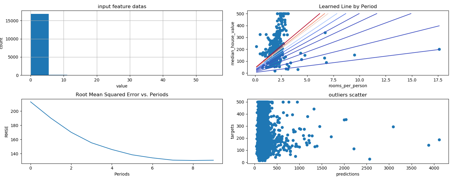
4.识别离群值
通过创建预测值与目标值的散点图来可视化模型效果。理想情况下,这些值将位于一条完全相关的对角线上。
查看 rooms_per_person 中值的分布情况,将这些异常情况追溯到源数据。
plt.figure(figsize=(15, 6))
plt.subplot(1, 2, 1)
plt.scatter(calibration_data["predictions"], calibration_data["targets"])
# x轴预测,y轴样本

重点关注偏离这条线的点。我们注意到这些点的数量相对较少。
如果我们绘制 rooms_per_person 的直方图,则会发现我们的输入数据中有少量离群值:
plt.subplot(1, 2, 2)
_ = california_housing_dataframe["rooms_per_person"].hist()
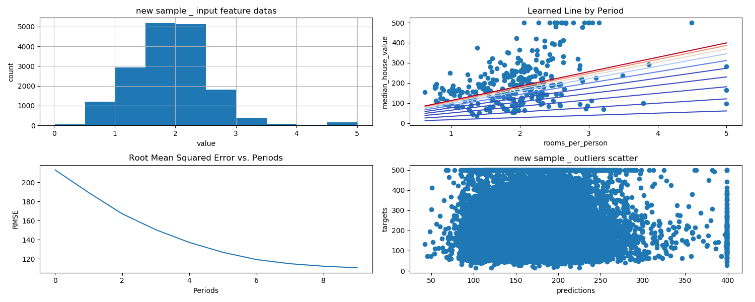
5.截取离群值
创建的直方图显示,大多数值都小于 5。
我们将 rooms_per_person 的值截取为 5,然后绘制直方图以再次检查结果。
california_housing_dataframe["rooms_per_person"] = (
    california_housing_dataframe["rooms_per_person"]).apply(lambda x: min(x, 5))

_ = california_housing_dataframe["rooms_per_person"].hist()
为了验证截取是否有效,我们再训练一次模型,并再次输出校准数据:
calibration_data = train_model(
    learning_rate=0.05,
    steps=500,
    batch_size=5,
    input_feature="rooms_per_person")

_ = plt.scatter(calibration_data["predictions"], calibration_data["targets"])
4.常用超参数
很多编码练习都包含以下超参数:
- steps:是指训练迭代的总次数。一步计算一批样本产生的损失,然后使用该值修改模型的权重一次。
- batch size:是指单步的样本数量(随机选择)。例如,SGD 的批量大小为 1。
以下公式成立:
5.方便变量
有些练习中会出现以下方便变量:
- periods:控制报告的粒度。例如,如果
periods设为 7 且steps设为 70,则练习将每 10 步(或 7 次)输出一次损失值。与超参数不同,我们不希望您修改periods的值。请注意,修改periods不会更改您的模型所学习的内容。
以下公式成立:

会话 (session)
维持 TensorFlow 程序中的状态(例如变量)。
skill 1:pycharm 注释 ctrl + /
skill 2: plt.figure 参数
skill 3: plt.subplot 参数
subplot(nrows, ncols, index, **kwargs)
参考