第一节 四格表资料的卡方分布
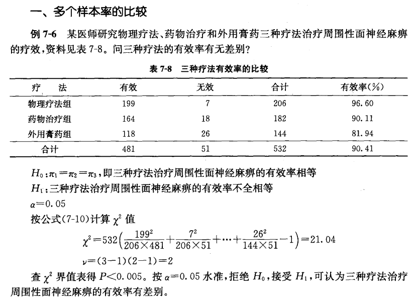
例7-1 两组降低颅内压有效率的比较
  组别    有效    无效    合计    有效率
试验组    99      5       104      95.2%
对照组    75      21      96        78.13
合计      174     26       200      87
卡方检验的步骤
H0 :pi1=pi2
H1 :Pi1 不等于 Pi2
> x<-c(99,75,5,21)
> dim(x)<-c(2,2)
> x
     [,1] [,2]
[1,]   99    5
[2,]   75   21
> chisq.test(x)

	Pearson's Chi-squared test with Yates' continuity correction

data:  x
X-squared = 11.392, df = 1, p-value = 0.0007375
P值<0.005 按a=0.05的水准,拒绝H0,接收H1,认为两组有效率不相等
对于四格表资料 通常规定:(n总样本数,T理论频数)
- 当n>40且所有的T>5时,用卡方检验的基本公式(套用chisp.test()),当p-value 接近检验水准a时。改用四格表资料的fisher确切概率法(fisher.test());
- 当n>40,但有1<T<5时,用四格表资料的fisher确切概率法
- 当n<40,或T<1时,用用四格表资料的fisher确切概率法
例7-2 两种药物治疗脑血管疾病有效率的比较
 组别    有效    无效    合计    有效率
胞碱组    46      6       52      88.46%
苷碱组    18      8(4.67) 36    69.23%
合计      64     14        78      82.05
其中 T(2,2)=(36*14)/78=4.67
运用fisher.test
> x<-c(46,18,6,8)
> dim(x)<-c(2,2)
> x
     [,1] [,2]
[1,]   46    6
[2,]   18    8
> fisher.test(x)

	Fisher's Exact Test for Count Data

data:  x
p-value = 0.05844
alternative hypothesis: true odds ratio is not equal to 1
95 percent confidence interval:
  0.879042 13.548216
sample estimates:
odds ratio
  3.347519
P值>0.05,不拒绝H0,还不能认为两种药品的有效率不等
第二节 配对四格表资料的卡方检验
例7-3 计数资料的配对设计常用于两种检验方法、培养方法、诊断方法的比较。
                  乳胶凝集法
免疫荧光法    阳性        阴性         合计
阳性            11        12            23
阴性            2         33             35
合计            13        45            58
运用Mcnemar test
> x<-c(11,2,12,33)
> dim(x)<-c(2,2)
> x
     [,1] [,2]
[1,]   11   12
[2,]    2   33
> mcnemar.test(x)

	McNemar's Chi-squared test with continuity correction

data:  x
McNemar's chi-squared = 5.7857, df = 1, p-value = 0.01616
第三节 四格表资料的fisher确切概率法
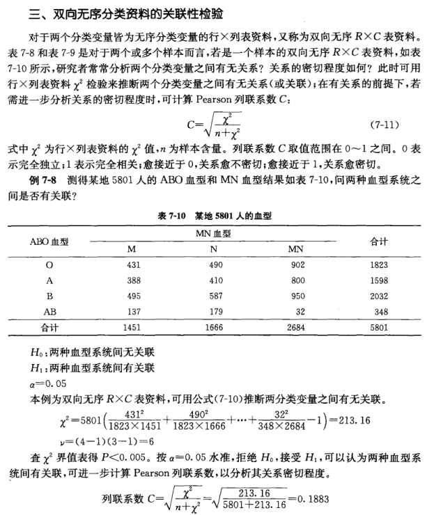
例7-4 当四格表资料中的n<40或T<1时,或者chisq.test 所得结果不准确时,运用fisher.test ,其理论依据是超几何分布(hypergeometric distribution)
        两组新生儿HBV感染率的比较
组别    阳性    阴性    合计    感染率
预防组    4       18    22        18.18%
非预防    5(3)  6      11        45.45
合计      9       24     33        27.27
样本总数33 小于40,
解法如下
> x<-c(4,5,18,6)
> dim(x)<-c(2,2)
> x
     [,1] [,2]
[1,]    4   18
[2,]    5    6
> chisq.test(x)

	Pearson's Chi-squared test with Yates' continuity correction

data:  x
X-squared = 1.5469, df = 1, p-value = 0.2136

Warning message:
In chisq.test(x) : Chi-squared近似算法有可能不准  # 在R语言中很明显的提示
> fisher.test(x)

	Fisher's Exact Test for Count Data

data:  x
p-value = 0.121
alternative hypothesis: true odds ratio is not equal to 1
95 percent confidence interval:
 0.03974151 1.76726409
sample estimates:
odds ratio
 0.2791061
例 7-5
        胆囊腺癌和胆囊腺瘤P53基因表达阳性率的比较
病种             阳性        阴性        合计
腺癌            6(3.5)      4            10
腺瘤            1(3.5)      9            10
合计            7            13            20
n<40 ,且 有两个格子的理论频数3.5<5 ,应用fisher确切概率法
> x<-c(6,1,4,9)
> dim(x)<-c(2,2)
> x
     [,1] [,2]
[1,]    6    4
[2,]    1    9
> fisher.test(x)

	Fisher's Exact Test for Count Data

data:  x
p-value = 0.05728
alternative hypothesis: true odds ratio is not equal to 1
95 percent confidence interval:
   0.9487882 684.4235629
sample estimates:
odds ratio
   11.6367
> #7-6 多个样本率的比较
> x<-c(199,164,118,7,18,26)
> dim(x)<-c(3,2)
> x
     [,1] [,2]
[1,]  199    7
[2,]  164   18
[3,]  118   26
> chisq.test(x)

	Pearson's Chi-squared test

data:  x
X-squared = 21.038, df = 2, p-value = 2.702e-05
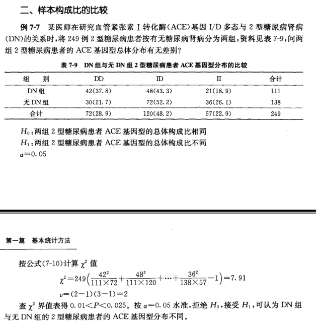
 #7-7 样本构成比 比较
> x<-c(42,30,48,72,21,36)
> dim(x)<-c(2,3)
> x
     [,1] [,2] [,3]
[1,]   42   48   21
[2,]   30   72   36
> chisq.test(x)

	Pearson's Chi-squared test

data:  x
X-squared = 7.9127, df = 2, p-value = 0.01913
> #7-8双向无序分类资料的关联性检验
> x<-c(431,388,495,137,490,410,587,179,902,800,950,32)
> dim(x)<-c(4,3)
> chisq.test(x)

	Pearson's Chi-squared test

data:  x
X-squared = 213.16, df = 6, p-value < 2.2e-16

> chisq.test(x)$statistic
X-squared
 213.1616
> a<-chisq.test(x)$statistic
> #列联系数
> C=sqrt(a/(5801+a));C
X-squared
0.1882638