一、对极几何
1.简介:多视图几何利用在不同视点拍摄的图像间关系研究相机或者特征之间的关系,而在多视图几何中最重要的基础就是双视图,如果已经有了一个场景的两个视图以及视图中的对应图像点,则依据相机位置关系,相机性质和三维场景点的位置可以得到图像点的几何关系约束,即对极几何。通过对极几何,我们可以在已知两幅图像中两点是对应关系的前提下,求解两个相机的相对位置和姿态。
若两个相机的光心分别为 C 和 C’ ,空间中的点为 X ,则有 五点共面,关系如下:
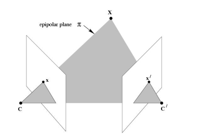
空间中的点X在两个像平面中的投影分别为x,x’ ,所以可得出C, C’,x,x’,X五点共面。
2.相关概念:
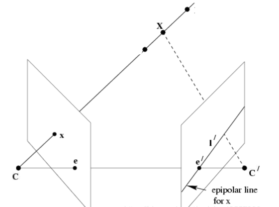
基线:两相机光心连线;
对极点 = 基线与像平面相交点 = 光心在另一幅图像中的投影;
对极平面 = 包含基线的平面;
对极线 = 对极平面与像平面的交线
3.对极约束:
点 x 和 x ’ 一定位于平面 π 上,而平面 π 可以利用基线 CC’ 和图像点 x 的反投影射线确定,点 x’ 又是右侧图像平面上的点,所以点 x’ 一定位于平面 π 与右侧图像平面的交线 l’ 上,直线 l’ 为点 x 的对极线,即点 x 的对应点 x’ 一定位于它的对极线上:
4.本质矩阵:
设 X 在 C,C’ 坐标系中的相对坐标分别 p,p’,R 为相机旋转矩阵,T 为光心位移向量,K 为相机内参矩阵:
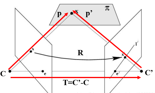
则有 p = R p’ + T ,又 C, C’, X 三点共面
可得 ( p - T ) T ( T × P ) = 0,将 p 代换可得:( RT p’ ) T ( T × p ) = 0
而 T × p = S p,(叉积 S 矩阵的秩为2,为反对称矩阵)
所以 ( R T p’ ) T ( S p ) = 0
( p’ T R )( S p ) = 0
得出 p’ E p = 0
E称为本质矩阵,本质矩阵描述了空间中的点在两个坐标系中的坐标对应关系
5.基础矩阵:
由上述已知 p’ E p = 0,且两个相机内参为 K, K’
所以 p = K -1 x, p’ = K’ -1 x’
代换得:
( K’ -1 x’ ) T E ( K -1 x ) = 0
所以 x’ T F x = 0
F称为基础矩阵 ,基础矩阵描述了空间中的点在两个像平面中的坐标对应关系,是对极几何的代数表达方式 ,在两幅图像中的任意匹配点对都满足上式。
我们可以将其用于图像特征点的 简化匹配或者去除错配特征 。
6.求解基础矩阵:
使用坐标系变换后的数据进行八点法计算
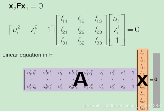
基本矩阵F对所有对应点x,x'都满足x‘(T)Fx=0 对应点可以先根据sift等算子检测出兴趣点,根据其灰度邻域的相似假设对应,再用RANSAC方法进行鲁棒估计,再进行非线性估计,最后引导匹配,进一步确定兴趣点的对应.不可能一下准确的找出来的.即使最后也不是完全准确的.
7.源代码:

# -*- coding: utf-8 -*-
from PIL import Image
from numpy import *
from pylab import *
import numpy as np
from PCV.geometry import camera
from PCV.geometry import homography
from PCV.geometry import sfm
from PCV.localdescriptors import sift
camera = reload(camera)
homography = reload(homography)
sfm = reload(sfm)
sift = reload(sift)
# Read features
im1 = array(Image.open('C:/Users/LE/PycharmProjects/untitled/yi/1.jpg'))
im2 = array(Image.open('C:/Users/LE/PycharmProjects/untitled/yi/2.jpg'))
sift.process_image('C:/Users/LE/PycharmProjects/untitled/yi/1.jpg', 'im1.sift')
l1, d1 =sift.read_features_from_file('im1.sift')
sift.process_image('C:/Users/LE/PycharmProjects/untitled/yi/2.jpg', 'im2.sift')
l2, d2 =sift.read_features_from_file('im2.sift')
matches = sift.match_twosided(d1, d2)
ndx = matches.nonzero()[0]
x1 = homography.make_homog(l1[ndx, :2].T)
ndx2 = [int(matches[i]) for i in ndx]
x2 = homography.make_homog(l2[ndx2, :2].T)
d1n = d1[ndx]
d2n = d2[ndx2]
x1n = x1.copy()
x2n = x2.copy()
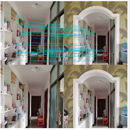
figure(figsize=(16,16))
sift.plot_matches(im1, im2, l1, l2, matches, True)
show()
#def F_from_ransac(x1, x2, model, maxiter=5000, match_threshold=1e-6):
def F_from_ransac(x1, x2, model, maxiter=5000, match_threshold=1e-6):
""" Robust estimation of a fundamental matrix F from point
correspondences using RANSAC (ransac.py from
http://www.scipy.org/Cookbook/RANSAC).
input: x1, x2 (3*n arrays) points in hom. coordinates. """
from PCV.tools import ransac
data = np.vstack((x1, x2))
d = 10 # 20 is the original
# compute F and return with inlier index
F, ransac_data = ransac.ransac(data.T, model,
8, maxiter, match_threshold, d, return_all=True)
return F, ransac_data['inliers']
# find F through RANSAC
model = sfm.RansacModel()
F, inliers = F_from_ransac(x1n, x2n, model, maxiter=5000, match_threshold=1e-1)
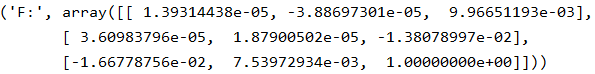
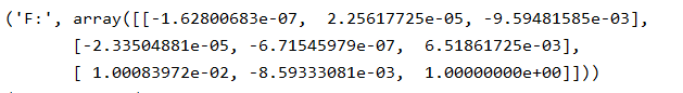
print("F:", F)
P1 = array([[1, 0, 0, 0], [0, 1, 0, 0], [0, 0, 1, 0]])
P2 = sfm.compute_P_from_fundamental(F)
print("P2:", P2)
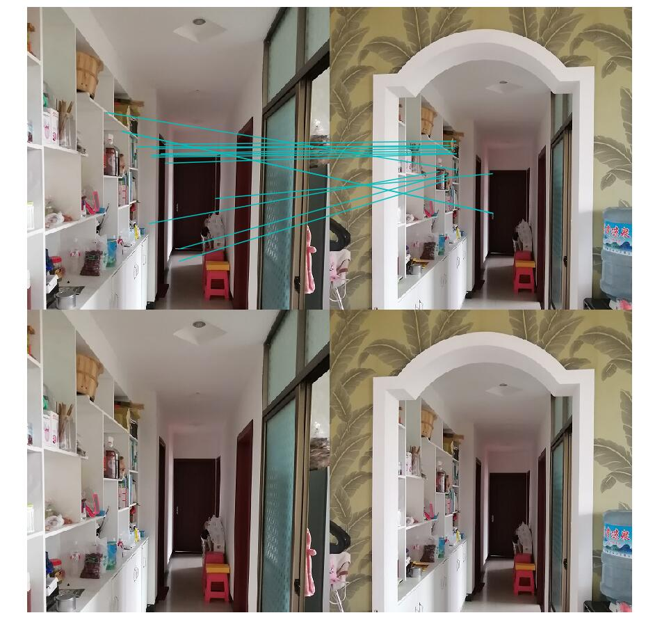
# triangulate inliers and remove points not in front of both cameras
X = sfm.triangulate(x1n[:, inliers], x2n[:, inliers], P1, P2)
# plot the projection of X
cam1 = camera.Camera(P1)
cam2 = camera.Camera(P2)
x1p = cam1.project(X)
x2p = cam2.project(X)
figure(figsize=(16, 16))
imj = sift.appendimages(im1, im2)
imj = vstack((imj, imj))
imshow(imj)
cols1 = im1.shape[1]
rows1 = im1.shape[0]
for i in range(len(x1p[0])):
if (0<= x1p[0][i]<cols1) and (0<= x2p[0][i]<cols1) and (0<=x1p[1][i]<rows1) and (0<=x2p[1][i]<rows1):
plot([x1p[0][i], x2p[0][i]+cols1],[x1p[1][i], x2p[1][i]],'c')
axis('off')
show()
d1p = d1n[inliers]
d2p = d2n[inliers]
# Read features
im3 = array(Image.open('C:/Users/LE/PycharmProjects/untitled/yi/2.jpg'))
sift.process_image('C:/Users/LE/PycharmProjects/untitled/yi/2.jpg', 'im2.sift')
l3, d3 = sift.read_features_from_file('im2.sift')
matches13 = sift.match_twosided(d1p, d3)
ndx_13 = matches13.nonzero()[0]
x1_13 = homography.make_homog(x1p[:, ndx_13])
ndx2_13 = [int(matches13[i]) for i in ndx_13]
x3_13 = homography.make_homog(l3[ndx2_13, :2].T)
figure(figsize=(16, 16))
imj = sift.appendimages(im1, im3)
imj = vstack((imj, imj))
imshow(imj)
cols1 = im1.shape[1]
rows1 = im1.shape[0]
for i in range(len(x1_13[0])):
if (0<= x1_13[0][i]<cols1) and (0<= x3_13[0][i]<cols1) and (0<=x1_13[1][i]<rows1) and (0<=x3_13[1][i]<rows1):
plot([x1_13[0][i], x3_13[0][i]+cols1],[x1_13[1][i], x3_13[1][i]],'c')
axis('off')
show()
P3 = sfm.compute_P(x3_13, X[:, ndx_13])
print("P1:", P1)
print("P2:", P2)
print("P3:", P3)
from pylab import *
from numpy import *
from scipy import linalg


def compute_P(x, X):
    """    Compute camera matrix from pairs of
        2D-3D correspondences (in homog. coordinates). """

    n = x.shape[1]
    if X.shape[1] != n:
        raise ValueError("Number of points don't match.")

    # create matrix for DLT solution
    M = zeros((3 * n, 12 + n))
    for i in range(n):
        M[3 * i, 0:4] = X[:, i]
        M[3 * i + 1, 4:8] = X[:, i]
        M[3 * i + 2, 8:12] = X[:, i]
        M[3 * i:3 * i + 3, i + 12] = -x[:, i]

    U, S, V = linalg.svd(M)

    return V[-1, :12].reshape((3, 4))


def triangulate_point(x1, x2, P1, P2):
    """ Point pair triangulation from
        least squares solution. """

    M = zeros((6, 6))
    M[:3, :4] = P1
    M[3:, :4] = P2
    M[:3, 4] = -x1
    M[3:, 5] = -x2

    U, S, V = linalg.svd(M)
    X = V[-1, :4]

    return X / X[3]


def triangulate(x1, x2, P1, P2):
    """    Two-view triangulation of points in
        x1,x2 (3*n homog. coordinates). """

    n = x1.shape[1]
    if x2.shape[1] != n:
        raise ValueError("Number of points don't match.")

    X = [triangulate_point(x1[:, i], x2[:, i], P1, P2) for i in range(n)]
    return array(X).T


def compute_fundamental(x1, x2):
    """    Computes the fundamental matrix from corresponding points
        (x1,x2 3*n arrays) using the 8 point algorithm.
        Each row in the A matrix below is constructed as
        [x'*x, x'*y, x', y'*x, y'*y, y', x, y, 1] """

    n = x1.shape[1]
    if x2.shape[1] != n:
        raise ValueError("Number of points don't match.")

    # build matrix for equations
    A = zeros((n, 9))
    for i in range(n):
        A[i] = [x1[0, i] * x2[0, i], x1[0, i] * x2[1, i], x1[0, i] * x2[2, i],
                x1[1, i] * x2[0, i], x1[1, i] * x2[1, i], x1[1, i] * x2[2, i],
                x1[2, i] * x2[0, i], x1[2, i] * x2[1, i], x1[2, i] * x2[2, i]]

    # compute linear least square solution
    U, S, V = linalg.svd(A)
    F = V[-1].reshape(3, 3)

    # constrain F
    # make rank 2 by zeroing out last singular value
    U, S, V = linalg.svd(F)
    S[2] = 0
    F = dot(U, dot(diag(S), V))

    return F / F[2, 2]


def compute_epipole(F):
    """ Computes the (right) epipole from a
        fundamental matrix F.
        (Use with F.T for left epipole.) """

    # return null space of F (Fx=0)
    U, S, V = linalg.svd(F)
    e = V[-1]
    return e / e[2]


def plot_epipolar_line(im, F, x, epipole=None, show_epipole=True):
    """ Plot the epipole and epipolar line F*x=0
        in an image. F is the fundamental matrix
        and x a point in the other image."""

    m, n = im.shape[:2]
    line = dot(F, x)

    # epipolar line parameter and values
    t = linspace(0, n, 100)
    lt = array([(line[2] + line[0] * tt) / (-line[1]) for tt in t])

    # take only line points inside the image
    ndx = (lt >= 0) & (lt < m)
    plot(t[ndx], lt[ndx], linewidth=2)

    if show_epipole:
        if epipole is None:
            epipole = compute_epipole(F)
        plot(epipole[0] / epipole[2], epipole[1] / epipole[2], 'r*')


def skew(a):
    """ Skew matrix A such that a x v = Av for any v. """

    return array([[0, -a[2], a[1]], [a[2], 0, -a[0]], [-a[1], a[0], 0]])


def compute_P_from_fundamental(F):
    """    Computes the second camera matrix (assuming P1 = [I 0])
        from a fundamental matrix. """

    e = compute_epipole(F.T)  # left epipole
    Te = skew(e)
    return vstack((dot(Te, F.T).T, e)).T


def compute_P_from_essential(E):
    """    Computes the second camera matrix (assuming P1 = [I 0])
        from an essential matrix. Output is a list of four
        possible camera matrices. """

    # make sure E is rank 2
    U, S, V = svd(E)
    if det(dot(U, V)) < 0:
        V = -V
    E = dot(U, dot(diag([1, 1, 0]), V))

    # create matrices (Hartley p 258)
    Z = skew([0, 0, -1])
    W = array([[0, -1, 0], [1, 0, 0], [0, 0, 1]])

    # return all four solutions
    P2 = [vstack((dot(U, dot(W, V)).T, U[:, 2])).T,
          vstack((dot(U, dot(W, V)).T, -U[:, 2])).T,
          vstack((dot(U, dot(W.T, V)).T, U[:, 2])).T,
          vstack((dot(U, dot(W.T, V)).T, -U[:, 2])).T]

    return P2


def compute_fundamental_normalized(x1, x2):
    """    Computes the fundamental matrix from corresponding points
        (x1,x2 3*n arrays) using the normalized 8 point algorithm. """

    n = x1.shape[1]
    if x2.shape[1] != n:
        raise ValueError("Number of points don't match.")

    # normalize image coordinates
    x1 = x1 / x1[2]
    mean_1 = mean(x1[:2], axis=1)
    S1 = sqrt(2) / std(x1[:2])
    T1 = array([[S1, 0, -S1 * mean_1[0]], [0, S1, -S1 * mean_1[1]], [0, 0, 1]])
    x1 = dot(T1, x1)

    x2 = x2 / x2[2]
    mean_2 = mean(x2[:2], axis=1)
    S2 = sqrt(2) / std(x2[:2])
    T2 = array([[S2, 0, -S2 * mean_2[0]], [0, S2, -S2 * mean_2[1]], [0, 0, 1]])
    x2 = dot(T2, x2)

    # compute F with the normalized coordinates
    F = compute_fundamental(x1, x2)

    # reverse normalization
    F = dot(T1.T, dot(F, T2))

    return F / F[2, 2]


class RansacModel(object):
    """ Class for fundmental matrix fit with ransac.py from
        http://www.scipy.org/Cookbook/RANSAC"""

    def __init__(self, debug=False):
        self.debug = debug

    def fit(self, data):
        """ Estimate fundamental matrix using eight
            selected correspondences. """

        # transpose and split data into the two point sets
        data = data.T
        x1 = data[:3, :8]
        x2 = data[3:, :8]

        # estimate fundamental matrix and return
        F = compute_fundamental_normalized(x1, x2)
        return F

    def get_error(self, data, F):
        """ Compute x^T F x for all correspondences,
            return error for each transformed point. """

        # transpose and split data into the two point
        data = data.T
        x1 = data[:3]
        x2 = data[3:]

        # Sampson distance as error measure
        Fx1 = dot(F, x1)
        Fx2 = dot(F, x2)
        denom = Fx1[0] ** 2 + Fx1[1] ** 2 + Fx2[0] ** 2 + Fx2[1] ** 2
        err = (diag(dot(x1.T, dot(F, x2)))) ** 2 / denom

        # return error per point
        return err


def F_from_ransac(x1, x2, model, maxiter=5000, match_theshold=1e-6):
    """ Robust estimation of a fundamental matrix F from point
        correspondences using RANSAC (ransac.py from
        http://www.scipy.org/Cookbook/RANSAC).

        input: x1,x2 (3*n arrays) points in hom. coordinates. """

    from PCV.tools import ransac

    data = vstack((x1, x2))

    # compute F and return with inlier index
    F, ransac_data = ransac.ransac(data.T, model, 8, maxiter, match_theshold, 20, return_all=True)
    return F, ransac_data['inliers']
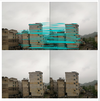
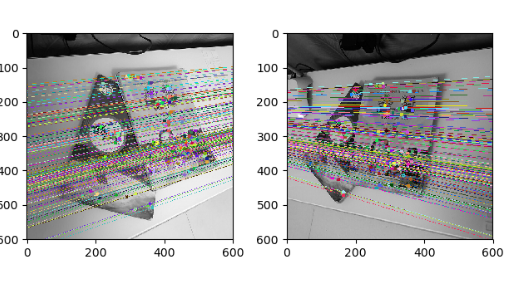
(1)左右拍摄,极点位于图像平面上
SIFT特征匹配:

ransac算法匹配:

8点算法:

基础矩阵:
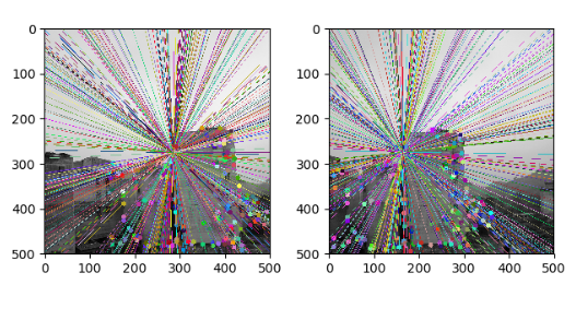
(2)像平面接近平行,极点位于无穷远
SIFT特征匹配
ransac算法匹配
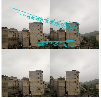
8点算法
基础矩阵:
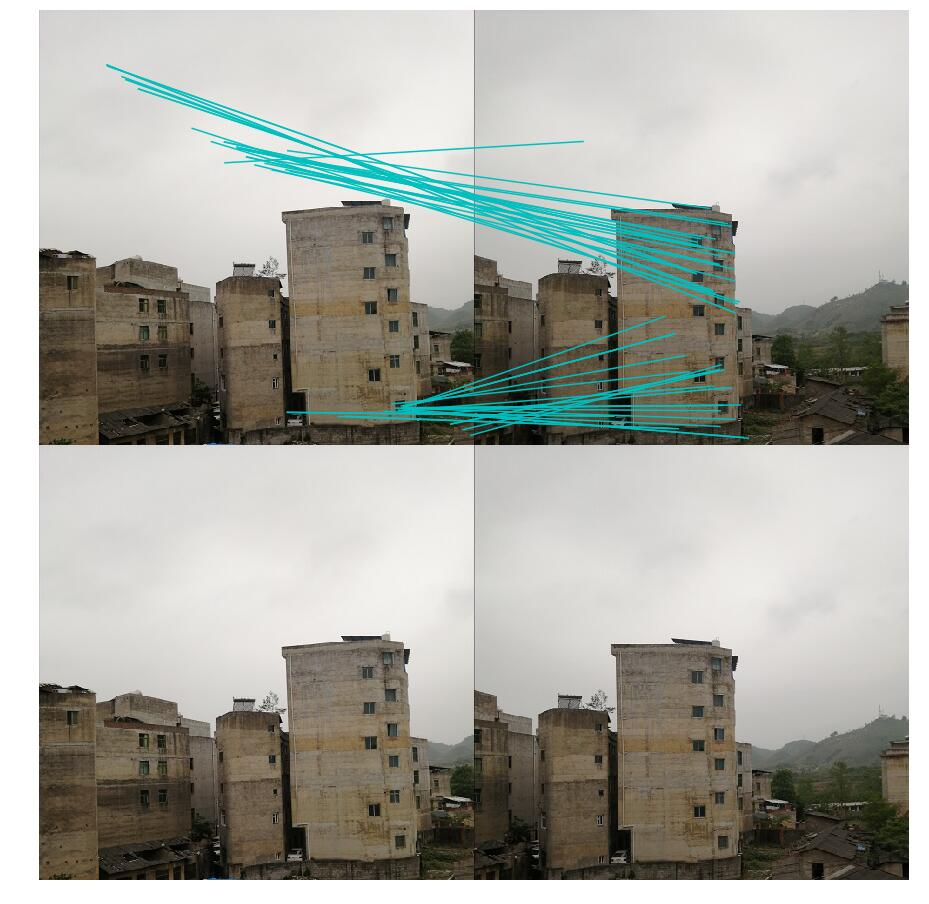
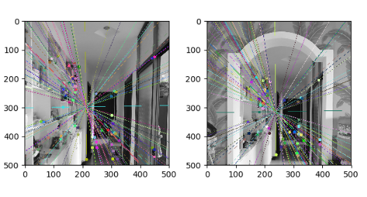
(3)图像拍摄位置位于前后
SIFT特征匹配
ransac算法匹配

8点算法
基础矩阵:

二、极点和极线
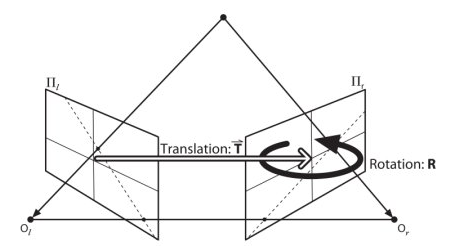
1.定义:由上述可假设O和O′ 是相机中心,则能看到在点处的左侧图像上可以看到右侧摄像机O′ 的投影。它称为极点。极点是穿过相机中心和图像平面的线的交点。左摄像机的极点也同理。在某些情况下,无法在图像中找到极点,它们可能位于图像外部(这意味着一个摄像机看不到另一个摄像机)。所有的极线都通过其极点。因此,要找到中心线的位置,我们可以找到许多中心线并找到它们的交点。要找到极点和极线我们需要另外两种成分,即基础矩阵(F)和本质矩阵(E),基础矩阵包含有关平移和旋转的信息,这些信息在全局坐标中描述了第二个摄像头相对于第一个摄像头的位置,如下图。
本质矩阵除包含有关两个摄像头的内参数,还包含与基本矩阵相同的信息,因此我们可以将两个摄像头的像素坐标关联起来。简而言之,基本矩阵F将一个图像中的点映射到另一图像中的线(上)。这是从两个图像的匹配点计算得出的。 至少需要8个这样的点才能找到基本矩阵(使用8点算法参考上述)。 选择更多点并使用RANSAC将获得更可靠的结果。
所以需要在两个图像之间找到尽可能多的匹配项,以找到基本矩阵,那就将SIFT描述符与基于FLANN的匹配器和比率测试结合使用。
2.源代码:
# -*- coding: utf-8 -*-
import numpy as np
import cv2 as cv
from matplotlib import pyplot as plt
img1 = cv.imread('C:/Users/LE/PycharmProjects/untitled/yi/1.jpg',0)  #索引图像 # left image
img2 = cv.imread('C:/Users/LE/PycharmProjects/untitled/yi/2.jpg',0) #训练图像 # right image
sift = cv.xfeatures2d.SIFT_create()
# 使用SIFT查找关键点和描述符
kp1, des1 = sift.detectAndCompute(img1,None)
kp2, des2 = sift.detectAndCompute(img2,None)
# FLANN 参数
FLANN_INDEX_KDTREE = 1
index_params = dict(algorithm = FLANN_INDEX_KDTREE, trees = 5)
search_params = dict(checks=50)
flann = cv.FlannBasedMatcher(index_params,search_params)
matches = flann.knnMatch(des1,des2,k=2)
good = []
pts1 = []
pts2 = []
# 根据Lowe的论文进行比率测试
for i,(m,n) in enumerate(matches):
    if m.distance < 0.8*n.distance:
        good.append(m)
        pts2.append(kp2[m.trainIdx].pt)
        pts1.append(kp1[m.queryIdx].pt)
pts1 = np.int32(pts1)
pts2 = np.int32(pts2)
F, mask = cv.findFundamentalMat(pts1,pts2,cv.FM_LMEDS)
# 我们只选择内点
pts1 = pts1[mask.ravel()==1]
pts2 = pts2[mask.ravel()==1]
def drawlines(img1,img2,lines,pts1,pts2):
    ''' img1 - 我们在img2相应位置绘制极点生成的图像
        lines - 对应的极点 '''
    r,c = img1.shape
    img1 = cv.cvtColor(img1,cv.COLOR_GRAY2BGR)
    img2 = cv.cvtColor(img2,cv.COLOR_GRAY2BGR)
    for r,pt1,pt2 in zip(lines,pts1,pts2):
        color = tuple(np.random.randint(0,255,3).tolist())
        x0,y0 = map(int, [0, -r[2]/r[1] ])
        x1,y1 = map(int, [c, -(r[2]+r[0]*c)/r[1] ])
        img1 = cv.line(img1, (x0,y0), (x1,y1), color,1)
        img1 = cv.circle(img1,tuple(pt1),5,color,-1)
        img2 = cv.circle(img2,tuple(pt2),5,color,-1)
    return img1,img2
# 在右图(第二张图)中找到与点相对应的极点,然后在左图绘制极线
lines1 = cv.computeCorrespondEpilines(pts2.reshape(-1,1,2), 2,F)
lines1 = lines1.reshape(-1,3)
img5,img6 = drawlines(img1,img2,lines1,pts1,pts2)
# 在左图(第一张图)中找到与点相对应的Epilines,然后在正确的图像上绘制极线
lines2 = cv.computeCorrespondEpilines(pts1.reshape(-1,1,2), 1,F)
lines2 = lines2.reshape(-1,3)
img3,img4 = drawlines(img2,img1,lines2,pts2,pts1)
plt.subplot(121),plt.imshow(img5)
plt.subplot(122),plt.imshow(img3)
plt.show()
3.运行结果:
(1)左右拍摄,极点位于图像平面上
(2)像平面接近平行,极点位于无穷远
(3)图像拍摄位置位于前后
三、总结
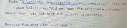
1.RANSAC 的稳健估计对于远近不同的图像集可能会最终遇到无法找到适配点对的情况,需要在调用时多次尝试对阈值(match_threshold=1e-3)进行调整以适用当前图像集;
2.对于较远的目标适配点对数量大,越容易增加错配无法去除的点对数量,对于较近的目标则相反;
3.错配情况时常发生且没有被剔除,甚至保留了错配很明显的点对而将较好的适配点剔除,这种现象与几乎完全相同的物体结构外观相对应,还有为了提高效率将图片分辨率进行降低处理的影响。
四、遇到的问题解决方法
问题1:
解决方法:
这是由于拍摄的图片匹配点不够造成的,重新拍摄匹配点较多的场景即可
问题2:
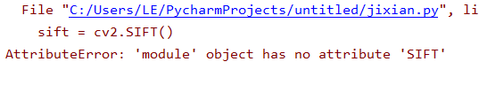
解决方法:
这是由于SIFT算法已经申请专利,OpenCV4以上的版本没有使用权限,所以要先降低OpenCV版本,在命令行下进行卸载操作:pip uninstall opencv-python和pip uninstall opencv-contrib-python
再安装低一点的版本:pip install opencv-python3.4.2.17和pip install opencv-contrib-python3.4.2.17