听说PyTorch比Tensorflow更加直观,更容易理解,就试一试
一、安装
打开官网
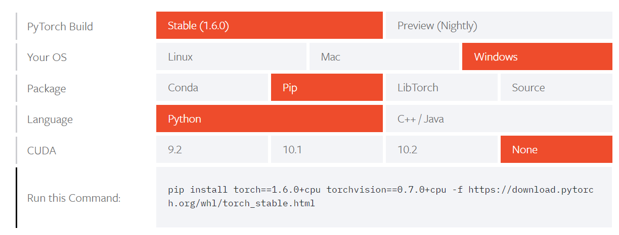
按自己的情况选择,我是在windows上且只使用cpu,下载最新的稳定版。
直接复制命令运行即可。
但是Torch有点大,直接用pip下载有点大。我们可以找到命令运行时所下载的xx.whl,拿出来用FDM等多线程下载器下载,然后再安装,例如
https://download.pytorch.org/whl/cpu/torch-1.6.0%2Bcpu-cp38-cp38-win_amd64.whl

>pip uninstall "torch-1.6.0+cpu-cp38-cp38-win_amd64.whl"
注意,torchvision版本与torch版本是对应的,不能随意匹配。所以我们用之前的命令把torchvision下完(已经下好的torch会自动跳过)
二、示例
import torch
import torch.nn.functional as F
import matplotlib.pyplot as plt

# torch.manual_seed(1)    # reproducible

x = torch.unsqueeze(torch.linspace(-1, 1, 100), dim=1)  # x data (tensor), shape=(100, 1)
y = x.pow(2) + 0.2*torch.rand(x.size())                 # noisy y data (tensor), shape=(100, 1)

# torch can only train on Variable, so convert them to Variable
# The code below is deprecated in Pytorch 0.4. Now, autograd directly supports tensors
# x, y = Variable(x), Variable(y)

# plt.scatter(x.data.numpy(), y.data.numpy())
# plt.show()


class Net(torch.nn.Module):
    def __init__(self, n_feature, n_hidden, n_output):
        super(Net, self).__init__()
        self.hidden = torch.nn.Linear(n_feature, n_hidden)   # hidden layer
        self.predict = torch.nn.Linear(n_hidden, n_output)   # output layer

    def forward(self, x):
        x = F.relu(self.hidden(x))      # activation function for hidden layer
        x = self.predict(x)             # linear output
        return x

net = Net(n_feature=1, n_hidden=10, n_output=1)     # define the network
print(net)  # net architecture

optimizer = torch.optim.SGD(net.parameters(), lr=0.2)
loss_func = torch.nn.MSELoss()  # this is for regression mean squared loss

plt.ion()   # something about plotting

for t in range(200):
    prediction = net(x)     # input x and predict based on x

    loss = loss_func(prediction, y)     # must be (1. nn output, 2. target)

    optimizer.zero_grad()   # clear gradients for next train
    loss.backward()         # backpropagation, compute gradients
    optimizer.step()        # apply gradients

    if t % 5 == 0:
        # plot and show learning process
        plt.cla()
        plt.scatter(x.data.numpy(), y.data.numpy())
        plt.plot(x.data.numpy(), prediction.data.numpy(), 'r-', lw=5)
        plt.text(0.5, 0, 'Loss=%.4f' % loss.data.numpy(), fontdict={'size': 20, 'color':  'red'})
        plt.pause(0.1)

plt.ioff()
plt.show()
三、其他
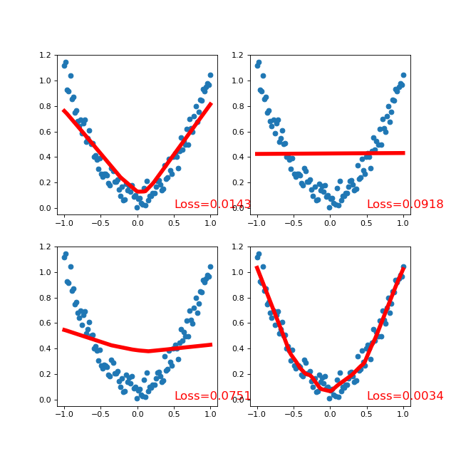
增加一层中间层,并使用激活函数,得到3个不同的net,进行横向对比
"""
View more, visit my tutorial page: https://morvanzhou.github.io/tutorials/
My Youtube Channel: https://www.youtube.com/user/MorvanZhou
Dependencies:
torch: 0.4
matplotlib
"""
import torch
from torch import nn
import torch.nn.functional as F
import matplotlib.pyplot as plt


x = torch.unsqueeze(torch.linspace(-1, 1, 100), dim=1)  # x data (tensor), shape=(100, 1)
y = x.pow(2) + 0.2*torch.rand(x.size())                 # noisy y data (tensor), shape=(100, 1)

# 1 10 1
class Net(torch.nn.Module):
    def __init__(self, n_feature, n_hidden, n_output):
        super(Net, self).__init__()
        self.hidden = torch.nn.Linear(n_feature, n_hidden)   # hidden layer
        self.predict = torch.nn.Linear(n_hidden, n_output)   # output layer

    def forward(self, x):
        x = F.relu(self.hidden(x))      # activation function for hidden layer
        x = self.predict(x)             # linear output
        return x

# 1 10 10 1
class simpleNet(nn.Module):
    """
    定义了一个简单的三层全连接神经网络,每一层都是线性的
    """
    def __init__(self, in_dim, n_hidden_1, n_hidden_2, out_dim):
        super(simpleNet, self).__init__()
        self.layer1 = nn.Linear(in_dim, n_hidden_1)
        self.layer2 = nn.Linear(n_hidden_1, n_hidden_2)
        self.layer3 = nn.Linear(n_hidden_2, out_dim)

    def forward(self, x):
        x = self.layer1(x)
        x = self.layer2(x)
        x = self.layer3(x)
        return x

class Activation_Net(nn.Module):
    """
    在上面的simpleNet的基础上,在每层的输出部分添加了激活函数
    """
    def __init__(self, in_dim, n_hidden_1, n_hidden_2, out_dim):
        super(Activation_Net, self).__init__()
        self.layer1 = nn.Sequential(nn.Linear(in_dim, n_hidden_1), nn.ReLU(True))
        self.layer2 = nn.Sequential(nn.Linear(n_hidden_1, n_hidden_2), nn.ReLU(True))
        self.layer3 = nn.Sequential(nn.Linear(n_hidden_2, out_dim))
        """
        这里的Sequential()函数的功能是将网络的层组合到一起。
        """

    def forward(self, x):
        x = self.layer1(x)
        x = self.layer2(x)
        x = self.layer3(x)
        return x

class Batch_Net(nn.Module):
    """
    在上面的Activation_Net的基础上,增加了一个加快收敛速度的方法——批标准化
    """
    def __init__(self, in_dim, n_hidden_1, n_hidden_2, out_dim):
        super(Batch_Net, self).__init__()
        self.layer1 = nn.Sequential(nn.Linear(in_dim, n_hidden_1), nn.BatchNorm1d(n_hidden_1), nn.ReLU(True))
        self.layer2 = nn.Sequential(nn.Linear(n_hidden_1, n_hidden_2), nn.BatchNorm1d(n_hidden_2), nn.ReLU(True))
        self.layer3 = nn.Sequential(nn.Linear(n_hidden_2, out_dim))

    def forward(self, x):
        x = self.layer1(x)
        x = self.layer2(x)
        x = self.layer3(x)
        return x


def Use(net):
    # print(net)
    optimizer = torch.optim.SGD(net.parameters(), lr=0.2)
    loss_func = torch.nn.MSELoss()  # this is for regression mean squared loss

    prediction = net(x)     # input x and predict based on x

    loss = loss_func(prediction, y)     # must be (1. nn output, 2. target)

    optimizer.zero_grad()   # clear gradients for next train
    loss.backward()         # backpropagation, compute gradients
    optimizer.step()

    return prediction, loss

def Draw(prediction, loss, ax):
    # plt.figure(figsize=(8,6), dpi=80)
    # ax = plt.subplot(1,2,num)
    ax.cla()
    ax.scatter(x.data.numpy(), y.data.numpy())
    ax.plot(x.data.numpy(), prediction.data.numpy(), 'r-', lw=5)
    ax.text(0.5, 0, 'Loss=%.4f' % loss.data.numpy(), fontdict={'size': 15, 'color':  'red'})
    plt.pause(0.1)


def start(ax1, ax2, ax3, ax4, net1, net2, net3, net4):
    for t in range(50):
        print("Generation %d" % t)
        prediction, loss = Use(net1)
        Draw(prediction, loss, ax1)
        prediction, loss = Use(net2)
        Draw(prediction, loss, ax2)
        prediction, loss = Use(net3)
        Draw(prediction, loss, ax3)
        prediction, loss = Use(net4)
        Draw(prediction, loss, ax4)


    plt.show()


plt.figure(figsize=(8, 8), dpi=80)
ax1 = plt.subplot(2,2,1)
ax2 = plt.subplot(2,2,2)
ax3 = plt.subplot(2,2,3)
ax4 = plt.subplot(2,2,4)

net1 = Net(n_feature=1, n_hidden=10, n_output=1)
net2 = simpleNet(in_dim=1, n_hidden_1=10, n_hidden_2=15, out_dim=1)
net3 = Activation_Net(in_dim=1, n_hidden_1=10, n_hidden_2=15, out_dim=1)
net4 = Batch_Net(in_dim=1, n_hidden_1=10, n_hidden_2=15, out_dim=1)

start(ax1, ax2, ax3, ax4, net1, net2, net3, net4)
参考链接:
1. https://github.com/MorvanZhou/PyTorch-Tutorial/blob/master/tutorial-contents/301_regression.py
2. https://blog.csdn.net/out_of_memory_error/article/details/81414986