P122, 这是IQR method课的第一次作业,需要统计检验,x和y是否显著的有线性关系。
Assignment 1
1) Find a small bivariate dataset (preferably from your
own discipline) and produce a scatterplot (this is easy
using any spreadsheet)
2) Use any statistics tool (a calculator, spreadsheet or
statistical package) to calculate the best fitting
regression line and test whether the population slope
(=B) is zero.
Notes:
1. Testing whether the population slope (=B) is zero is
different to whether the estimated slope (=b) is zero.
2. Instructions for loading and using the Analysis
Toolpak in Excel: <https://support.office.com/en-us/article/load-theanalysis-
toolpak-in-excel-6a63e598-cd6d-42e3-9317-6b40ba1a66b4>
入门:散点图、线性拟合、拟合参数slope
进阶:统计检验,多重矫正FDR
基本概念:
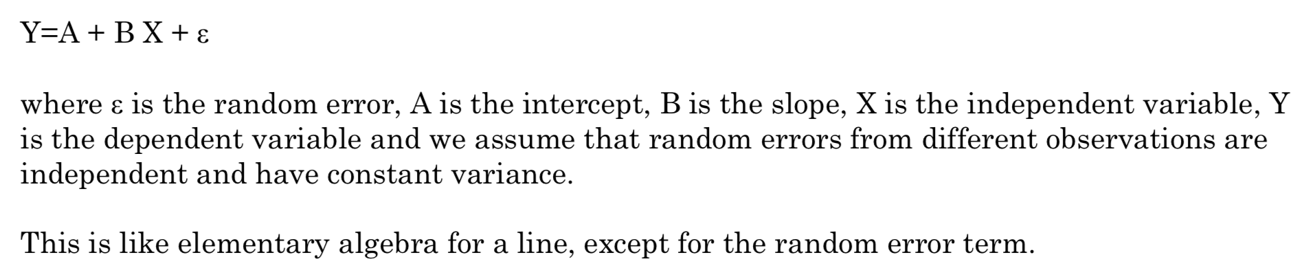
这和基本的代数一样,只是统计更加严谨,把误差纳入到模型中了。
怎么估计A和B呢?
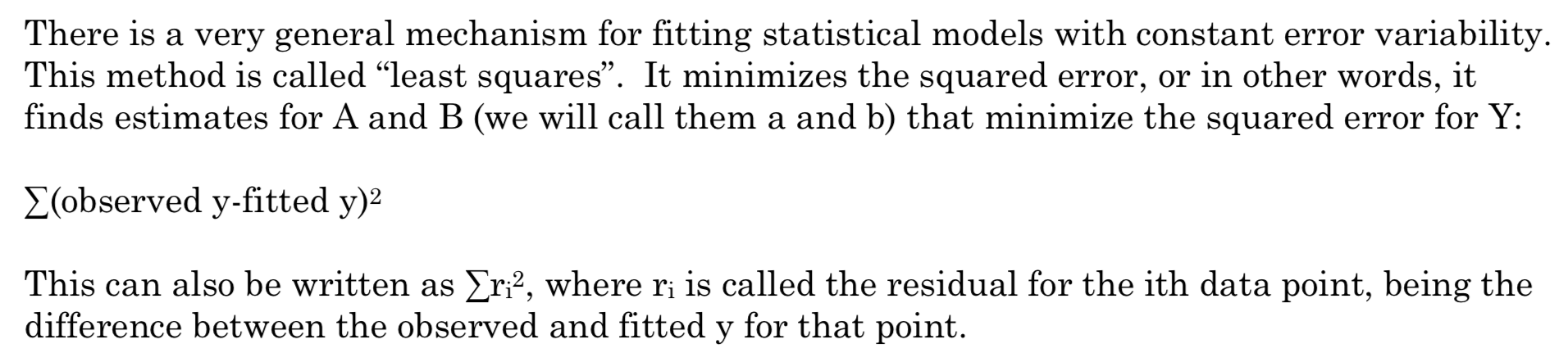
A和B可以看做是群体的参数,a和b可以看做是样本的估计参数,我们的方法是通过使残差最小来估计出a和b。
如果我们假设误差项服从正态分布,那么我们就可以对slope斜率进行统计推断。
我们可以构造出一个关于b的统计量,它会服从t分布。
这部分还是看耶鲁大学的教程吧:Inference in Linear Regression
如果只是应用的话,知道怎么用R求显著性就行了。
入门R代码
height <- c(176, 154, 138, 196, 132, 176, 181, 169, 150, 175)
bodymass <- c(82, 49, 53, 112, 47, 69, 77, 71, 62, 78)
plot(bodymass, height)
plot(bodymass, height, pch = 16, cex = 1.3, col = "blue", main = "HEIGHT PLOTTED AGAINST BODY MASS", xlab = "BODY MASS (kg)", ylab = "HEIGHT (cm)")

进阶
eruption.lm = lm(eruptions ~ waiting, data=faithful)
summary(eruption.lm)
help(summary.lm)
Call:
lm(formula = eruptions ~ waiting, data = faithful)

Residuals:
    Min      1Q  Median      3Q     Max
-1.2992 -0.3769  0.0351  0.3491  1.1933

Coefficients:
            Estimate Std. Error t value Pr(>|t|)
(Intercept) -1.87402    0.16014   -11.7   <2e-16 ***
waiting      0.07563    0.00222    34.1   <2e-16 ***
---
Signif. codes:  0 ’***’ 0.001 ’**’ 0.01 ’*’ 0.05 ’.’ 0.1 ’ ’ 1

Residual standard error: 0.497 on 270 degrees of freedom
Multiple R-squared: 0.811,      Adjusted R-squared: 0.811
F-statistic: 1.16e+03 on 1 and 270 DF,  p-value: <2e-16
Decide whether there is a significant relationship between the variables in the linear regression model of the data set faithful at .05 significance level.
NULL hypothesis: no relationship between x and y, so the slope is zero.
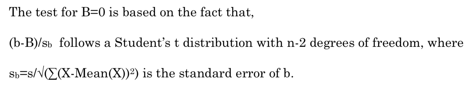
假设误差服从正态分布,基于零假设,我们要检验以下统计量是否显著。
统计量:(b-B)/sb follows a Student’s t distribution with n-2 degrees of freedom, where sb=s/√(∑(X-Mean(X))2) is the standard error of b.
进阶:多项回归,多重检验
多次回归以后专门开一贴,以下讲多重检验multiple testing。
Lecture 10: Multiple Testing - PPT通俗易懂
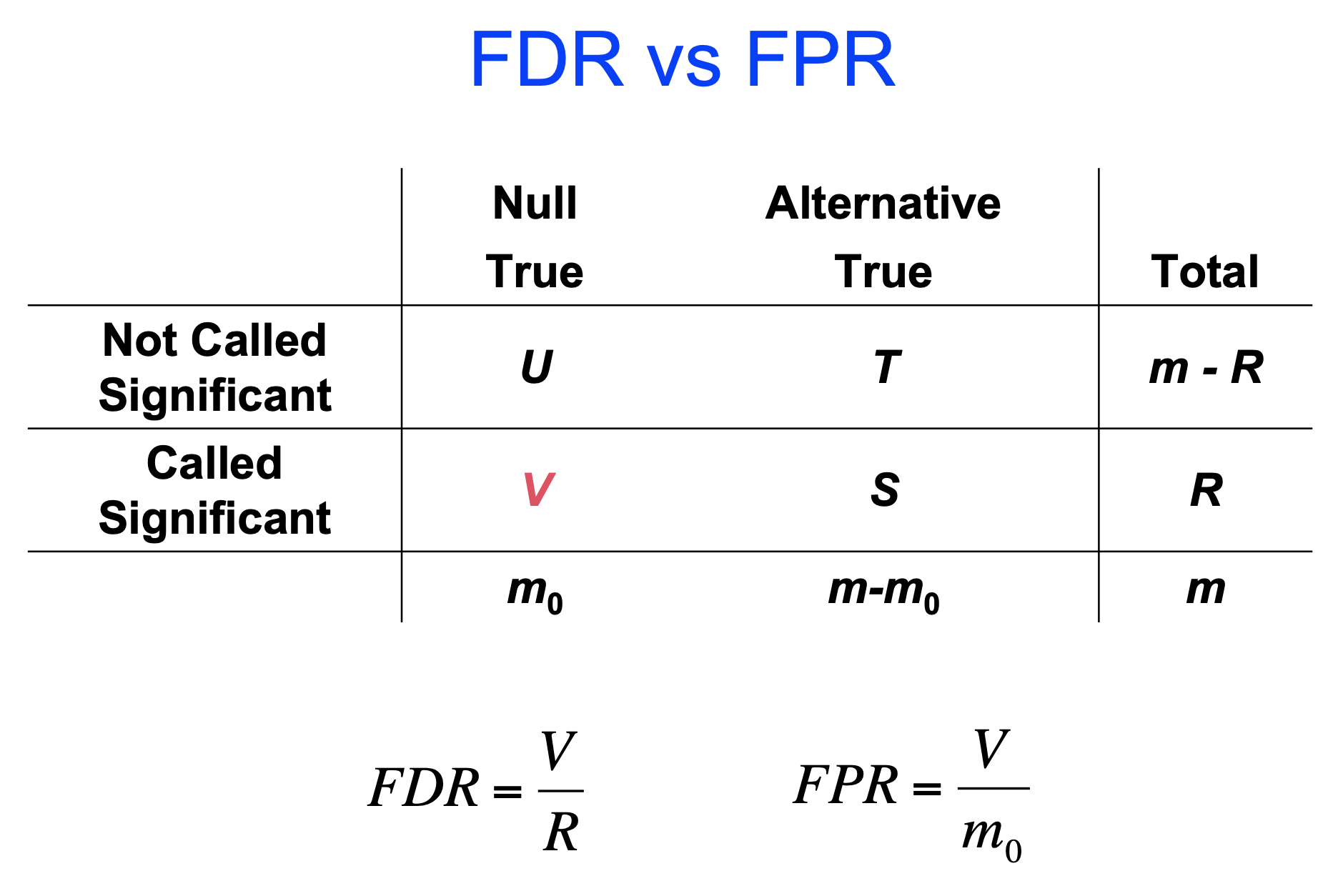
所有的问题都是围绕着多重和error(就是一个2X2的表,根据检验和真实,有四种可能)的:
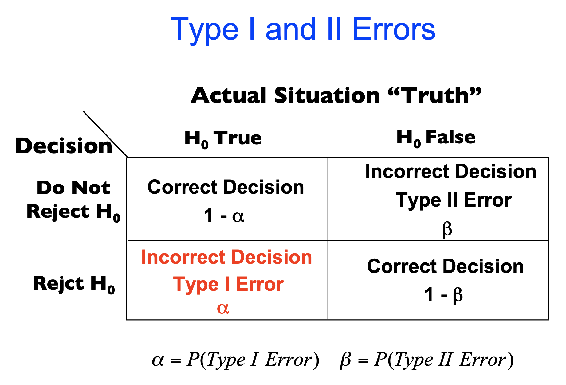
做一次检验,我们犯第一类错误(应该是真的,我们拒绝了,又叫错误拒绝率)为a,犯第二类错误(应该是假的,我们接受了,又叫纳伪率)为b。
那么,我们做基因差异表达,对每一个基因做一次检验,有3万多个基因,我们至少犯1次第一类错误的概率是多少呢?1-(a)2
为了使我们整体犯第一类错的概率效率0.05,我们必须要进行多重矫正。
方法1:
Bonferroni,直接把a 0.05除以次数,比如1万,来设立显著性阈值,这样会极大地增大第二类错误,我们会漏掉大量有用的信息。
方法2:
FDR,就是错误发现率,假/真阳性比例,就是显著水平里的真显著和假显著的比例。千万不要和假阳性率搞混了。
做法很简答,把我们检测出来的显著的结果按p-value排列一下,去掉后面5%不太显著的结果。FDR的计算方法很多,BH最为常用。
最熟悉的例子就是:生物信息学里的GO富集分析,一次检验是指我们的gene list与一个GO term做超几何分布检验,然而GO terms那么多,我们必须矫正,以控制错误率。
另一个就是一鸣的组会讲的回归问题的拟合,我们拟合了很多次,需要对p-value做矫正,看PPT。
medium专题
这个非常值得一看,回归里的系数和p-value分别是什么含义。
How to Interpret Regression Analysis Results: P-values and Coefficients
null hypothesis:coefficient is 0,如果p-value小于0.05,我们就可以拒绝零假设。
multiple testing
Benjamini and Hochberg's method
aggregated FDR
FDR with group info
Hu, James X., Hongyu Zhao, and Harrison H. Zhou. "False discovery rate control with groups." Journal of the American Statistical Association 105.491 (2010): 1215-1227.
pak说:这个太重要了,对于大数据时代的统计而言。
一般情况下:我们可以认为Q value = FDR = adjusted p value,即三者是一个东西,虽然有些定义上的细微区别,但是问题也不大。
参考:浅谈多重检验校正FDR
待续~