更新:又用了一段时间,发现是真的好用,可惜就是服务器上装不上,只能在Mac上用了。
核心代码很少:
library(ggbio)

# hg19
library(EnsDb.Hsapiens.v75)
ensdb <- EnsDb.Hsapiens.v75

options(repr.plot.width=15, repr.plot.height=9)
autoplot(ensdb, GeneNameFilter("PKM")) +
    # ME of exon 9 and 10
    geom_vline(xintercept = c(72492996,72494795), linetype="dashed", color = "red", size=0.5) +
    theme_bw()

# hg38
library(EnsDb.Hsapiens.v86)
ensdb <- EnsDb.Hsapiens.v86

options(repr.plot.width=15, repr.plot.height=9)
autoplot(ensdb, GeneNameFilter("PKM")) +
    # ME of exon 9 and 10
    geom_vline(xintercept = c(72200655,72202454), linetype="dashed", color = "red", size=0.5) +
    theme_bw()
版本问题
ensembl版本列表:https://asia.ensembl.org/info/website/archives/assembly.html
NCBI上的基因都有hg19和hg38两个版本的坐标,可以辅助使用。
只搞基因表达还没啥,现在搞到了isoform,即exon级别,想要随时查看底层的数据就很困难了。
比如下面就是AS分析的结果,想要手动去检查数据,完全不知所措。

一个AS event的命名:
isoform1=junction:chr11:237145-244160:+|isoform2=junction:chr11:237145-238997:+@exon:chr11:238998-239076:+@junction:chr11:239077-244160:+
里面都是具体的基因组位置了,UCSC Genome Browser和IGV都无法胜任,因为无法标明单个碱基的位置。
这时候就发现了一个神器,ggbio: An R implementation for extending the Grammar of Graphics for Genomic Data
http://bioconductor.org/packages/release/bioc/html/ggbio.html
https://github.com/tengfei/ggbio
另一个发现:spliceclust
下面描述其具体用法:
library(ggbio)
library(Homo.sapiens)
class(Homo.sapiens)
data(genesymbol, package = "biovizBase")
wh <- genesymbol[c("PTBP1")]
wh <- range(wh, ignore.strand = TRUE)
p.txdb <- autoplot(Homo.sapiens, which = wh)
p.txdb
options(repr.plot.width=8, repr.plot.height=4)
p.txdb
autoplot(Homo.sapiens, which = wh, label.color = "black", color = "brown", fill = "brown")
autoplot(Homo.sapiens, which = wh, gap.geom = "chevron")
autoplot(Homo.sapiens, which = wh, stat = "reduce")
--------------------------------------------------
library(EnsDb.Hsapiens.v75)
ensdb <- EnsDb.Hsapiens.v75
autoplot(ensdb, GeneNameFilter("PTBP1"))
options(repr.plot.width=10, repr.plot.height=6)
autoplot(ensdb, GeneNameFilter("PTBP1"))
autoplot(ensdb, ~ symbol == "PTBP1", names.expr="gene_name")
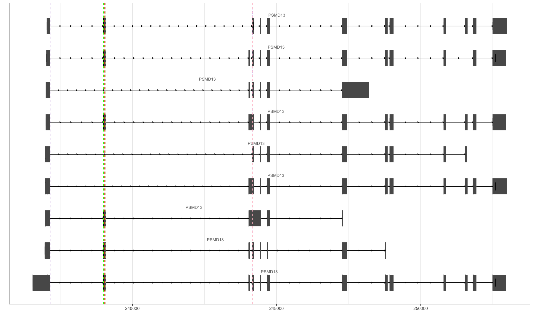
autoplot(ensdb, ~ symbol == "PSMD13", names.expr="gene_name")
--------------------------------------------------
## We specify "*" as strand, thus we query for genes encoded on both strands
gr <- GRanges(seqnames = 11, IRanges(238998, 239076), strand = "+")
autoplot(ensdb, GRangesFilter(gr), names.expr = "gene_name")
options(repr.plot.width=15, repr.plot.height=9)
autoplot(ensdb, GRangesFilter(gr), names.expr = "gene_name") +
#geom_vline(xintercept = c(237145,244160), linetype="dashed", color = "blue", size=0.5) +
#geom_vline(xintercept = c(237145,238997), linetype="dashed", color = "red", size=0.5) +
geom_vline(xintercept = c(238998,239076), linetype="dashed", color = "green", size=0.5) +
#geom_vline(xintercept = c(239077,244160), linetype="dashed", color = "black", size=0.5) +
theme_bw()
最后的图片:
稍微搞清楚了的概念:
junction:从一个exon的结束到另一个exon的起点,这就是一个junction,俗称跳跃点、接合点,因为这两个点注定要连在一起。
AS event:一个可变剪切的事件,如何定义呢?一个exon,以及三个junction即可定义,要满足等式相等原则【一个完整的junction = 一个sub junction + exon + 一个sub junction】,即一个exon的inclusion/exclusion。
可视化的威力真是无穷,直观明了的揭示了数据之间的关系,这是肉眼直接看数据所做不到的!!!