PCA(principal component analysis )即主成分分析,是一种常用的降维方法。
假设我们用降维操作处理一个二维的数据集(二维压缩成一维):

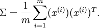
在这个数据集上,我们可以计算出两个方向,我们称为主方向u1和次方向u2,其中u1的值是数据集协方差矩阵的最大特征值对应的特征向量,u2是次大特征值对应的特征向量。数据集的协方差矩阵(这个符号很像求和但不是):
我们现在用U=[u1 u2]处理x,由矩阵变换可知这相当于一个旋转变换:
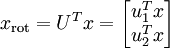
上图中x轴为u1,y轴为u2
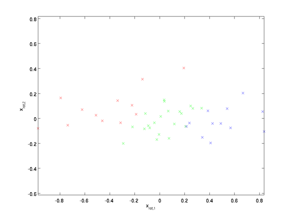
为了降维,我们只选择一个维度,比如u1,那么
这里就有一个问题了,我们怎么选择去掉的维度呢?这就要引入维度重要性的判断标准了:

 是特征值按递减排列。这里的意思是数据每个维度对整体的贡献可以用特征值的大小来衡量,越大的特征值贡献越大,越应该保留。
Whitening:白化指的是对特征进行预处理,使得数据满足:
1.不同特征间相关性尽量小
2.各特征的协方差为一
参考练习:http://deeplearning.stanford.edu/wiki/index.php/Exercise:PCA_in_2D
close all

%%================================================================
%% Step 0: Load data
%  We have provided the code to load data from pcaData.txt into x.
%  x is a 2 * 45 matrix, where the kth column x(:,k) corresponds to
%  the kth data point.Here we provide the code to load natural image data into x.
%  You do not need to change the code below.

x = load('pcaData.txt','-ascii');
figure(1);
scatter(x(1, :), x(2, :));
title('Raw data');


%%================================================================
%% Step 1a: Implement PCA to obtain U
%  Implement PCA to obtain the rotation matrix U, which is the eigenbasis
%  sigma.

% -------------------- YOUR CODE HERE --------------------
u = zeros(size(x, 1)); % You need to compute this
[m n]=size(x);
x_mean = mean(x,2);
x_submean = x-repmat(x_mean,1,n);
sigma = (1.0/m)*x*x';
[u s v] = svd(sigma);


% --------------------------------------------------------
hold on
plot([0 u(1,1)], [0 u(2,1)]);
plot([0 u(1,2)], [0 u(2,2)]);
scatter(x(1, :), x(2, :));
hold off

%%================================================================
%% Step 1b: Compute xRot, the projection on to the eigenbasis
%  Now, compute xRot by projecting the data on to the basis defined
%  by U. Visualize the points by performing a scatter plot.

% -------------------- YOUR CODE HERE --------------------
xRot = zeros(size(x)); % You need to compute this

xRot = u'*x;

% --------------------------------------------------------

% Visualise the covariance matrix. You should see a line across the
% diagonal against a blue background.
figure(2);
scatter(xRot(1, :), xRot(2, :));
title('xRot');

%%================================================================
%% Step 2: Reduce the number of dimensions from 2 to 1.
%  Compute xRot again (this time projecting to 1 dimension).
%  Then, compute xHat by projecting the xRot back onto the original axes
%  to see the effect of dimension reduction

% -------------------- YOUR CODE HERE --------------------
k = 1; % Use k = 1 and project the data onto the first eigenbasis
xHat = zeros(size(x)); % You need to compute this
xHat = u*([u(:,1),zeros(m,1)]'*x);

% --------------------------------------------------------
figure(3);
scatter(xHat(1, :), xHat(2, :));
title('xHat');


%%================================================================
%% Step 3: PCA Whitening
%  Complute xPCAWhite and plot the results.

epsilon = 1e-5;
% -------------------- YOUR CODE HERE --------------------
xPCAWhite = zeros(size(x)); % You need to compute this
xPCAWhite = diag(1./sqrt(diag(s)+epsilon))*u'*x;


% --------------------------------------------------------
figure(4);
scatter(xPCAWhite(1, :), xPCAWhite(2, :));
title('xPCAWhite');

%%================================================================
%% Step 3: ZCA Whitening
%  Complute xZCAWhite and plot the results.

% -------------------- YOUR CODE HERE --------------------
xZCAWhite = zeros(size(x)); % You need to compute this
xZCAWhite = u*diag(1./sqrt(diag(s)+epsilon))*u'*x;

% --------------------------------------------------------
figure(5);
scatter(xZCAWhite(1, :), xZCAWhite(2, :));
title('xZCAWhite');

%% Congratulations! When you have reached this point, you are done!
%  You can now move onto the next PCA exercise. :)
参考练习
http://deeplearning.stanford.edu/wiki/index.php/Exercise:PCA_and_Whitening
%%================================================================
%% Step 0a: Load data
%  Here we provide the code to load natural image data into x.
%  x will be a 144 * 10000 matrix, where the kth column x(:, k) corresponds to
%  the raw image data from the kth 12x12 image patch sampled.
%  You do not need to change the code below.

x = sampleIMAGESRAW();
figure('name','Raw images');
randsel = randi(size(x,2),200,1); % A random selection of samples for visualization
display_network(x(:,randsel));

%%================================================================
%% Step 0b: Zero-mean the data (by row)
%  You can make use of the mean and repmat/bsxfun functions.

% -------------------- YOUR CODE HERE --------------------
[m n] = size(x);
x_mean = mean(x,1);
x_submean = x - repmat(x_mean,m,1);
x = x_submean;

%%================================================================
%% Step 1a: Implement PCA to obtain xRot
%  Implement PCA to obtain xRot, the matrix in which the data is expressed
%  with respect to the eigenbasis of sigma, which is the matrix U.


% -------------------- YOUR CODE HERE --------------------
xRot = zeros(size(x)); % You need to compute this
[n m] = size(x);
sigma = (1.0/m)*x*x';
[u s v] =svd(sigma);
xRot = u'*x;

%%================================================================
%% Step 1b: Check your implementation of PCA
%  The covariance matrix for the data expressed with respect to the basis U
%  should be a diagonal matrix with non-zero entries only along the main
%  diagonal. We will verify this here.
%  Write code to compute the covariance matrix, covar.
%  When visualised as an image, you should see a straight line across the
%  diagonal (non-zero entries) against a blue background (zero entries).

% -------------------- YOUR CODE HERE --------------------
covar = zeros(size(x, 1)); % You need to compute this
covar = (1./m)*xRot*xRot';
% Visualise the covariance matrix. You should see a line across the
% diagonal against a blue background.
figure('name','Visualisation of covariance matrix');
imagesc(covar);

%%================================================================
%% Step 2: Find k, the number of components to retain
%  Write code to determine k, the number of components to retain in order
%  to retain at least 99% of the variance.

% -------------------- YOUR CODE HERE --------------------
k = 0; % Set k accordingly
s_1 = diag(s);
s_sum = sum(s_1);
for k=1:m
    if sum(s(1:k)./s_sum) >= 0.99
        break;
    end
end
k = length(s_1((cumsum(s_1)/sum(s_1))<=0.99));

%%================================================================
%% Step 3: Implement PCA with dimension reduction
%  Now that you have found k, you can reduce the dimension of the data by
%  discarding the remaining dimensions. In this way, you can represent the
%  data in k dimensions instead of the original 144, which will save you
%  computational time when running learning algorithms on the reduced
%  representation.
%
%  Following the dimension reduction, invert the PCA transformation to produce
%  the matrix xHat, the dimension-reduced data with respect to the original basis.
%  Visualise the data and compare it to the raw data. You will observe that
%  there is little loss due to throwing away the principal components that
%  correspond to dimensions with low variation.

% -------------------- YOUR CODE HERE --------------------
xHat = zeros(size(x));  % You need to compute this
xHat = u*[u(:,1:k)'*x;zeros(n-k,m)];


% Visualise the data, and compare it to the raw data
% You should observe that the raw and processed data are of comparable quality.
% For comparison, you may wish to generate a PCA reduced image which
% retains only 90% of the variance.

figure('name',['PCA processed images ',sprintf('(%d / %d dimensions)', k, size(x, 1)),'']);
display_network(xHat(:,randsel));
figure('name','Raw images');
display_network(x(:,randsel));

%%================================================================
%% Step 4a: Implement PCA with whitening and regularisation
%  Implement PCA with whitening and regularisation to produce the matrix
%  xPCAWhite.

epsilon = 0.1;
xPCAWhite = zeros(size(x));

% -------------------- YOUR CODE HERE --------------------
xPCAWhite = diag(1./sqrt(diag(s)+epsilon))*u'*x;
figure('name','xPCAWhitened');
display_network(xPCAWhite(:,randsel));
%%================================================================
%% Step 4b: Check your implementation of PCA whitening
%  Check your implementation of PCA whitening with and without regularisation.
%  PCA whitening without regularisation results a covariance matrix
%  that is equal to the identity matrix. PCA whitening with regularisation
%  results in a covariance matrix with diagonal entries starting close to
%  1 and gradually becoming smaller. We will verify these properties here.
%  Write code to compute the covariance matrix, covar.
%
%  Without regularisation (set epsilon to 0 or close to 0),
%  when visualised as an image, you should see a red line across the
%  diagonal (one entries) against a blue background (zero entries).
%  With regularisation, you should see a red line that slowly turns
%  blue across the diagonal, corresponding to the one entries slowly
%  becoming smaller.

% -------------------- YOUR CODE HERE --------------------
covar = (1./m)*xPCAWhite*xPCAWhite';
% Visualise the covariance matrix. You should see a red line across the
% diagonal against a blue background.
figure('name','Visualisation of covariance matrix');
imagesc(covar);

%%================================================================
%% Step 5: Implement ZCA whitening
%  Now implement ZCA whitening to produce the matrix xZCAWhite.
%  Visualise the data and compare it to the raw data. You should observe
%  that whitening results in, among other things, enhanced edges.

xZCAWhite = zeros(size(x));

% -------------------- YOUR CODE HERE --------------------
xZCAWhite = u*xPCAWhite;

% Visualise the data, and compare it to the raw data.
% You should observe that the whitened images have enhanced edges.
figure('name','ZCA whitened images');
display_network(xZCAWhite(:,randsel));
figure('name','Raw images');
display_network(x(:,randsel));
版权声明:本文为博主原创文章,未经博主允许不得转载。