知识点
第一类生产线平衡问题,第二类生产线平衡问题
整数线性规划模型,+Leapms模型,直接求解,CPLEX求解
装配生产线平衡问题 (The Assembly Line Balancing Problem)
装配生产线又叫做组装生产线, 是把产品的工艺做串行生产安排的流水生产线。一个产品的组装需要不同的工序来完成,且工序之间有先后次序要求。
下表是Jackson, J. R. . (1956)给出一个产品工序的装配次序要求:
| 工序 | 执行时长 | 紧前工序 |
| 1 | 6 | -- |
| 2 | 2 | 1 |
| 3 | 5 | 1 |
| 4 | 7 | 1 |
| 5 | 1 | 1 |
| 6 | 2 | 2 |
| 7 | 3 | 3,4,5 |
| 8 | 6 | 6 |
| 9 | 5 | 7 |
| 10 | 5 | 8 |
| 11 | 4 | 10,9 |
上表也可以用有向图表示:
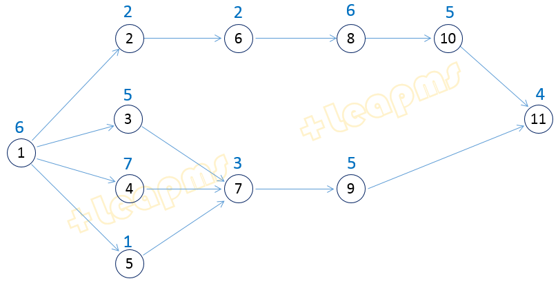
生产线平衡问题的目的是:把工序划分成工作站,且满足工序紧前要求。优化目标有两种:(1)在生产节拍被指定时使得工作站数量最少;或(2)在工作站数量被限定情况下使得生产节拍最小。
前一种目标被称为第一类生产线平衡问题,后一种目标被称为第二类生产线平衡问题。
第二类问题生产线平衡问题的建模
(1)问题
已知工作站共有m=5个,工序共有n=11个,极小化生产节拍。
(2)有向图的表达
有向图可以表达为节点的点对集合,例如 e={ 1 2, 1 3, 1 4,...,10 11}
第k条边的前后两个顶点一般被写成 a[k], 和 b[k]。第k条边被记为 (a[k], b[k])
边的数目 ne 是 e 中元素数除以2,即:ne=_$(e)/2
(3)决策变量
设 x[i][j] 为0-1变量,表示工序j是否被分配给工作站i。其中i=1,...,m; j=1,...,n。
(4)依赖变量
设变量c为生产线的节拍
(5)目标是极小化生产节拍,即:
minimize c
(6)约束1: 每个工序被分配给且仅被分配给一个工作站:
sum{i=1,...,m} x[i][j] =1 | j =1,...,n
(7)约束2:节拍大于等于任何一个工作站的执行时长:
c >= sum{j=1,...,n}x[i][j]t[j] | i=1,...,m
(8)约束3:对任何边k,如果其后节点b[k]被分配到工作站i,则其前节点 a[k] 必须被分配到 j=1,...,i 中的某个节点,即:
x[i][b[k]] <= sum{j=1,...,i}x[j][a[k]] | i=1,...,m;k=1,...,ne
第二类问题生产线平衡问题的+leapms模型
//第二类生产线平衡问题
minimize  c

subject to
    sum{i=1,...,m} x[i][j] =1 | j =1,...,n
    c >= sum{j=1,...,n}x[i][j]t[j] | i=1,...,m
    x[i][b[k]]<=sum{j=1,...,i}x[j][a[k]]|i=1,...,m;k=1,...,ne

where
    m,n,ne are integers
    t[j] is a number | j=1,...,n
    e is a set
    a[k],b[k] is an integer|k=1,...,ne
    c is a variable of number
    x[i][j] is a variable of binary|i=1,...,m;j=1,...,n

data
    m=5
    n=11
    t={6 2 5 7 1 2 3 6 5 5 4}
    e={
      1 2
      1 3
      1 3
      1 5
      2 6
      3 7
      4 7
      5 7
      6 8
      7 9
      8 10
      9 11
      10 11
    }

data_relation
  ne=_$(e)/2
  a[k]=e[2k-1]|k=1,...,ne
  b[k]=e[2k]|k=1,...,ne
第二类问题生产线平衡问题的模型求解
Welcome to +Leapms ver 1.1(162260) Teaching Version  -- an LP/LMIP modeling and
solving tool.欢迎使用利珀 版本1.1(162260) Teaching Version  -- LP/LMIP 建模和求
解工具.

+Leapms>load
 Current directory is "ROOT".
 .........
        p2.leap
 .........
please input the filename:p2
================================================================
1:  //第二类生产线平衡问题
2:  minimize  c
3:
4:  subject to
5:      sum{i=1,...,m} x[i][j] =1 | j =1,...,n
6:      c >= sum{j=1,...,n}x[i][j]t[j] | i=1,...,m
7:      x[i][b[k]]<=sum{j=1,...,i}x[j][a[k]]|i=1,...,m;k=1,...,ne
8:
9:  where
10:      m,n,ne are integers
11:      t[j] is a number | j=1,...,n
12:      e is a set
13:      a[k],b[k] is an integer|k=1,...,ne
14:      c is a variable of number
15:      x[i][j] is a variable of binary|i=1,...,m;j=1,...,n
16:
17:  data
18:      m=5
19:      n=11
20:      t={6 2 5 7 1 2 3 6 5 5 4}
21:      e={
22:        1 2
23:        1 3
24:        1 3
25:        1 5
26:        2 6
27:        3 7
28:        4 7
29:        5 7
30:        6 8
31:        7 9
32:        8 10
33:        9 11
34:        10 11
35:      }
36:  data_relation
37:    ne=_$(e)/2
38:    a[k]=e[2k-1]|k=1,...,ne
39:    b[k]=e[2k]|k=1,...,ne
40:
================================================================
>>end of the file.
Parsing model:
1D
2R
3V
4O
5C
6S
7End.
..................................
number of variables=56
number of constraints=81
..................................
+Leapms>mip
relexed_solution=9.2; number_of_nodes_branched=0; memindex=(2,2)
 nbnode=230;  memindex=(24,24) zstar=13; GB->zi=10
The Problem is solved to optimal as an MIP.
找到整数规划的最优解.非零变量值和最优目标值如下:
  .........
    c* =10
    x1_1* =1
    x1_5* =1
    x2_2* =1
    x2_6* =1
    x2_8* =1
    x3_3* =1
    x3_10* =1
    x4_4* =1
    x4_7* =1
    x5_9* =1
    x5_11* =1
  .........
    Objective*=10
  .........
+Leapms>
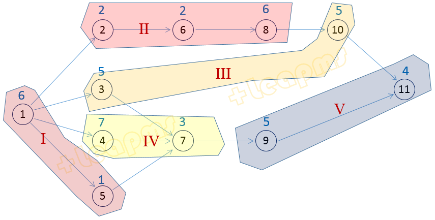
上面的结果显示, 目标值即最小节拍为10, 分配方案是: 工序1,5分配在工作站1, 工序2,6,8 分配在工作站2, 工序3,10 分配在工作站3, 工序4,7分配在工作站4, 工序9,11分配在工作站5。
第二类生产线平衡问题求解结果图示
第二类生产线平衡问题的+Leapms-Latex数学概念模型
在+Leapms环境下,使用 “latex"命令可以把上面的+Leapms模型直接转换为如下Latex格式的数学概念模型。

第一类生产线平衡问题
由求解第2类生产线平衡问题知道,工作站数是5时,最小节拍是10。假设如果将节拍上限增加到10,问是否能够减小工作站数目。
第一类生产线平衡问题的建模
第一类生产线平衡问题的数学模型见Ritt, M. , & Costa, A. M. . (2015)。
第一类生产线平衡问题的+Leapms模型
//第一类生产线平衡问题
minimize  sum{i=1,...,m}y[i]

subject to
    sum{i=1,...,m} x[i][j] =1 | j =1,...,n
    y[i]c >= sum{j=1,...,n}x[i][j]t[j] | i=1,...,m
    x[i][b[k]]<=sum{j=1,...,i}x[j][a[k]]|i=1,...,m;k=1,...,ne
    y[i]<=y[i-1]|i=2,...,m

where
    m,n,ne are integers
    t[j] is a number | j=1,...,n
    e is a set
    a[k],b[k] is an integer|k=1,...,ne
    c is a number
    x[i][j] is a variable of binary|i=1,...,m;j=1,...,n
    y[i] is a variable of binary|i=1,...,m

data
    m=6
    n=11
    c=12
    t={6 2 5 7 1 2 3 6 5 5 4}
    e={
      1 2
      1 3
      1 3
      1 5
      2 6
      3 7
      4 7
      5 7
      6 8
      7 9
      8 10
      9 11
      10 11
    }
data_relation
  ne=_$(e)/2
  a[k]=e[2k-1]|k=1,...,ne
  b[k]=e[2k]|k=1,...,ne
第一类生产线平衡问题的模型求解
Welcome to +Leapms ver 1.1(162260) Teaching Version  -- an LP/LMIP modeling and
solving tool.欢迎使用利珀 版本1.1(162260) Teaching Version  -- LP/LMIP 建模和求
解工具.

+Leapms>load
 Current directory is "ROOT".
 .........
        p1.leap
        p2.leap
 .........
please input the filename:p1
1:  //第一类生产线平衡问题
2:  minimize  sum{i=1,...,m}y[i]
3:
4:  subject to
5:      sum{i=1,...,m} x[i][j] =1 | j =1,...,n
6:      y[i]c >= sum{j=1,...,n}x[i][j]t[j] | i=1,...,m
7:      x[i][b[k]]<=sum{j=1,...,i}x[j][a[k]]|i=1,...,m;k=1,...,ne
8:      y[i]<=y[i-1]|i=2,...,m
9:
10:  where
11:      m,n,ne are integers
12:      t[j] is a number | j=1,...,n
13:      e is a set
14:      a[k],b[k] is an integer|k=1,...,ne
15:      c is a number
16:      x[i][j] is a variable of binary|i=1,...,m;j=1,...,n
17:      y[i] is a variable of binary|i=1,...,m
18:
19:  data
20:      m=6
21:      n=11
22:      c=12
23:      t={6 2 5 7 1 2 3 6 5 5 4}
24:      e={
25:        1 2
26:        1 3
27:        1 3
28:        1 5
29:        2 6
30:        3 7
31:        4 7
32:        5 7
33:        6 8
34:        7 9
35:        8 10
36:        9 11
37:        10 11
38:      }
39:  data_relation
40:    ne=_$(e)/2
41:    a[k]=e[2k-1]|k=1,...,ne
42:    b[k]=e[2k]|k=1,...,ne
43:
>>end of the file.
Parsing model:
1D
2R
3V
4O
5C
6S
7End.
===========================================
number of variables=72
number of constraints=100
int_obj=0
===========================================

+Leapms>mip
relexed_solution=3.83333; number_of_nodes_branched=0; memindex=(2,2)
 nbnode=117;  memindex=(12,12) zstar=5.22619; GB->zi=6
 nbnode=314;  memindex=(38,38) zstar=5.625; GB->zi=6
 nbnode=587;  memindex=(24,24) zstar=5.01852; GB->zi=5
 nbnode=861;  memindex=(26,26) zstar=4.25; GB->zi=5
 nbnode=1128;  memindex=(22,22) zstar=3.83333; GB->zi=5
 nbnode=1395;  memindex=(38,38) zstar=3.83333; GB->zi=5
 nbnode=1680;  memindex=(40,40) zstar=6; GB->zi=5
 nbnode=1959;  memindex=(46,46) zstar=6; GB->zi=5
 nbnode=2230;  memindex=(30,30) zstar=3.9246; GB->zi=5
 nbnode=2487;  memindex=(26,26) zstar=4.44444; GB->zi=5
 nbnode=2774;  memindex=(36,36) zstar=4.16667; GB->zi=4
 nbnode=2971;  memindex=(20,20) zstar=3.83333; GB->zi=4
 nbnode=3149;  memindex=(26,26) zstar=4.16667; GB->zi=4
 nbnode=3343;  memindex=(36,36) zstar=3.91667; GB->zi=4
 nbnode=3546;  memindex=(20,20) zstar=4.04167; GB->zi=4
The Problem is solved to optimal as an MIP.
找到整数规划的最优解.非零变量值和最优目标值如下:
  .........
    x1_1* =1
    x1_2* =1
    x1_6* =1
    x2_5* =1
    x2_8* =1
    x2_10* =1
    x3_3* =1
    x3_4* =1
    x4_7* =1
    x4_9* =1
    x4_11* =1
    y1* =1
    y2* =1
    y3* =1
    y4* =1
  .........
    Objective*=4
  .........
+Leapms>
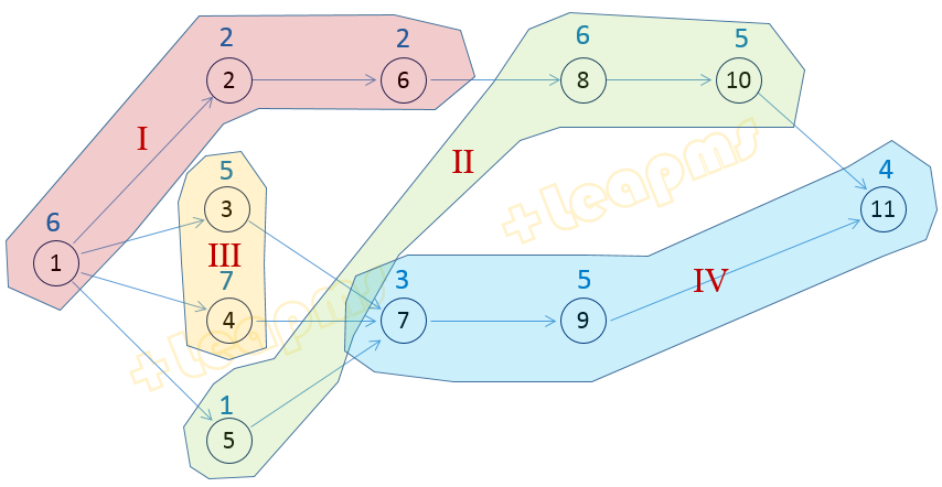
结果显示工作站数可减少到4。分配方式如下面的图示。
第一类生产线平衡问题求解结果图示
第一类生产线平衡问题的CPLEX求解
在+Leapms环境中输入cplex命令即可触发在另外窗口内启动CPLEX求解器对模型进行求解:
+Leapms>cplex
  You must have licience for Ilo Cplex, otherwise you will violate
  corresponding copyrights, continue(Y/N)?
  你必须有Ilo Cplex软件的授权才能使用此功能,否则会侵犯相应版权,
  是否继续(Y/N)?y
+Leapms>
Tried aggregator 1 time.
MIP Presolve eliminated 24 rows and 3 columns.
MIP Presolve modified 71 coefficients.
Reduced MIP has 76 rows, 69 columns, and 362 nonzeros.
Reduced MIP has 69 binaries, 0 generals, 0 SOSs, and 0 indicators.
Presolve time = 0.11 sec. (0.33 ticks)
Found incumbent of value 6.000000 after 0.20 sec. (0.40 ticks)
Probing fixed 15 vars, tightened 0 bounds.
Probing changed sense of 1 constraints.
Probing time = 0.00 sec. (0.18 ticks)
Cover probing fixed 1 vars, tightened 0 bounds.
Tried aggregator 1 time.
MIP Presolve eliminated 20 rows and 16 columns.
MIP Presolve modified 45 coefficients.
Reduced MIP has 56 rows, 53 columns, and 247 nonzeros.
Reduced MIP has 53 binaries, 0 generals, 0 SOSs, and 0 indicators.
Presolve time = 0.01 sec. (0.21 ticks)
Probing fixed 1 vars, tightened 0 bounds.
Probing time = 0.02 sec. (0.11 ticks)
Tried aggregator 1 time.
MIP Presolve eliminated 3 rows and 1 columns.
MIP Presolve modified 12 coefficients.
Reduced MIP has 53 rows, 52 columns, and 230 nonzeros.
Reduced MIP has 52 binaries, 0 generals, 0 SOSs, and 0 indicators.
Presolve time = 0.02 sec. (0.15 ticks)
Probing time = 0.00 sec. (0.10 ticks)
Clique table members: 207.
MIP emphasis: balance optimality and feasibility.
MIP search method: dynamic search.
Parallel mode: deterministic, using up to 4 threads.
Root relaxation solution time = 0.05 sec. (0.33 ticks)

        Nodes                                         Cuts/
   Node  Left     Objective  IInf  Best Integer    Best Bound    ItCnt     Gap

*     0+    0                            6.0000        4.0000            33.33%
*     0+    0                            5.0000        4.0000            20.00%
      0     0        4.0000    21        5.0000        4.0000       54   20.00%
*     0+    0                            4.0000        4.0000             0.00%
      0     0        cutoff              4.0000        4.0000       54    0.00%
Elapsed time = 0.45 sec. (1.85 ticks, tree = 0.00 MB, solutions = 3)

Root node processing (before b&c):
  Real time             =    0.45 sec. (1.85 ticks)
Parallel b&c, 4 threads:
  Real time             =    0.00 sec. (0.00 ticks)
  Sync time (average)   =    0.00 sec.
  Wait time (average)   =    0.00 sec.
                          ------------
Total (root+branch&cut) =    0.45 sec. (1.85 ticks)
Solution status = Optimal
Solution value  = 4
        x1_1=1
        x1_2=1
        x1_5=1
        x1_6=1
        x2_8=1
        x2_10=1
        x3_3=1
        x3_4=1
        x4_7=1
        x4_9=1
        x4_11=1
        y1=1
        y2=1
        y3=1
        y4=1
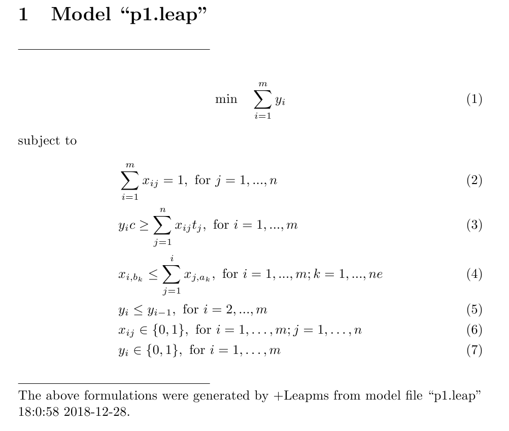
第一类生产线平衡问题的+Leapms-Latex数学概念模型
在+Leapms环境下,使用 “latex"命令可以把上面的+Leapms模型直接转换为如下Latex格式的数学概念模型
参考文献
[1] Jackson, J. R. . (1956). A computing procedure for a line balancing problem. Management Science, 2(3), 261-271.
[2] Ritt, M. , & Costa, A. M. . (2015). Improved integer programming models for simple assembly line balancing, and related problems. International Transactions in Operational Research, 19(8), 455-455.