
代码:
%% ++++++++++++++++++++++++++++++++++++++++++++++++++++++++++++++++++++++++++++++++++++++++
%% Output Info about this m-file
fprintf('
***********************************************************
');
fprintf(' <DSP using MATLAB> Problem 5.18
');
banner();
%% ++++++++++++++++++++++++++++++++++++++++++++++++++++++++++++++++++++++++++++++++++++++++
% -------------------------------------------------------------------------------------
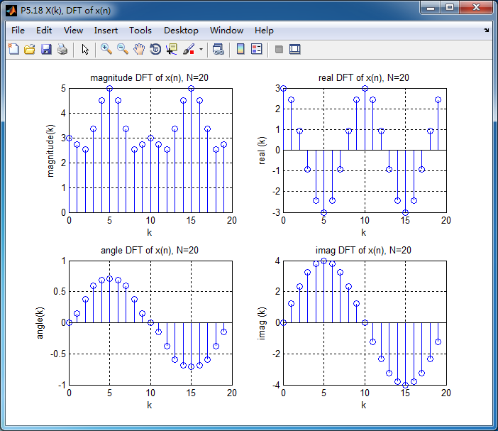
% X(k) is 20-point DFTs of Complex-valued sequence x(n)
% X(k) = [3cos(0.2pi*k) + j4sin(0.1pi*k)][u(k)-u(k-20)]
% N = 20 k=[0:19]
%
% xccs = [x(n)+ x*((-n))]/2 xcca = [x(n) - x*((-n))]/2
% DFT[xccs] = real(X(k)) DFT[xcca] = j*imag(X(k))
% -------------------------------------------------------------------------------------
k1 = [0:19];
Xk_DFT = (3*cos(0.2*pi*k1) + j*4*sin(0.1*pi*k1)) .* (stepseq(0,min(k1),max(k1))-stepseq(20,min(k1),max(k1)));
N1 = length(Xk_DFT); % length is 10
magXk_DFT = abs( [ Xk_DFT ] ); % DFT magnitude
angXk_DFT = angle( [Xk_DFT] )/pi; % DFT angle
realXk_DFT = real(Xk_DFT); imagXk_DFT = imag(Xk_DFT);
figure('NumberTitle', 'off', 'Name', 'P5.18 X(k), DFT of x(n)')
set(gcf,'Color','white');
subplot(2,2,1); stem(k1, magXk_DFT);
xlabel('k'); ylabel('magnitude(k)');
title('magnitude DFT of x(n), N=20'); grid on;
subplot(2,2,3); stem(k1, angXk_DFT);
%axis([-N/2, N/2, -0.5, 50.5]);
xlabel('k'); ylabel('angle(k)');
title('angle DFT of x(n), N=20'); grid on;
subplot(2,2,2); stem(k1, realXk_DFT);
xlabel('k'); ylabel('real (k)');
title('real DFT of x(n), N=20'); grid on;
subplot(2,2,4); stem(k1, imagXk_DFT);
%axis([-N/2, N/2, -0.5, 50.5]);
xlabel('k'); ylabel('imag (k)');
title('imag DFT of x(n), N=20'); grid on;
[xn] = idft(Xk_DFT, N1); % Complex-valued sequence
n = [0 : N1-1];
% +++++++++++++++++++++++++++++++++++++++++++++++++++++++++++++++++++++++
% x(n) decomposition into circular-conjugate-symmetric and
% circular-conjugate-antisymmetric parts
% +++++++++++++++++++++++++++++++++++++++++++++++++++++++++++++++++++++++
[xccs, xcca] = circevod_cv(xn);
% +++++++++++++++++++++++++++++++++++++++++++++++++++++++
% DFT(k) of xccs and xcca, k=[0:N1-1]
% +++++++++++++++++++++++++++++++++++++++++++++++++++++++
k1 = [0:19];
Xk_CCS_DFT = dft(xccs, length(xccs));
Xk_CCA_DFT = dft(xcca, length(xcca));
N1 = length(Yk_DFT); % length is 10
magXk_CCS_DFT = abs( [ Xk_CCS_DFT ] ); % DFT magnitude
angXk_CCS_DFT = angle( [Xk_CCS_DFT] )/pi; % DFT angle
realXk_CCS_DFT = real(Xk_CCS_DFT);
imagXk_CCS_DFT = imag(Xk_CCS_DFT);
magXk_CCA_DFT = abs( [ Xk_CCA_DFT ] ); % DFT magnitude
angXk_CCA_DFT = angle( [Xk_CCA_DFT] )/pi; % DFT angle
realXk_CCA_DFT = real(Xk_CCA_DFT);
imagXk_CCA_DFT = imag(Xk_CCA_DFT);
figure('NumberTitle', 'off', 'Name', 'P5.18 DFT(k) of xccs(n)')
set(gcf,'Color','white');
subplot(2,2,1); stem(k1, magXk_CCS_DFT);
xlabel('k'); ylabel('magnitude(k)');
title('magnitude DFT of xccs(n), N=20'); grid on;
subplot(2,2,3); stem(k1, angXk_CCS_DFT);
xlabel('k'); ylabel('angle(k)');
title('angle DFT of xccs(n), N=20'); grid on;
subplot(2,2,2); stem(k1, realXk_CCS_DFT);
xlabel('k'); ylabel('real (k)');
title('real DFT of xccs(n), N=20'); grid on;
subplot(2,2,4); stem(k1, imagXk_CCS_DFT);
%axis([-N/2, N/2, -0.5, 50.5]);
xlabel('k'); ylabel('imag (k)');
title('imag DFT of xccs(n), N=20'); grid on;
figure('NumberTitle', 'off', 'Name', 'P5.18 DFT(k) of xcca(n)')
set(gcf,'Color','white');
subplot(2,2,1); stem(k1, magXk_CCA_DFT);
xlabel('k'); ylabel('magnitude(k)');
title('magnitude DFT of xcca(n), N=20'); grid on;
subplot(2,2,3); stem(k1, angXk_CCA_DFT);
xlabel('k'); ylabel('angle(k)');
title('angle DFT of xcca(n), N=20'); grid on;
subplot(2,2,2); stem(k1, realXk_CCA_DFT);
xlabel('k'); ylabel('real (k)');
title('real DFT of xcca(n), N=20'); grid on;
subplot(2,2,4); stem(k1, imagXk_CCA_DFT);
%axis([-N/2, N/2, -0.5, 50.5]);
xlabel('k'); ylabel('imag (k)');
title('imag DFT of xcca(n), N=20'); grid on;
% --------------------------------------------------------------
% Verify
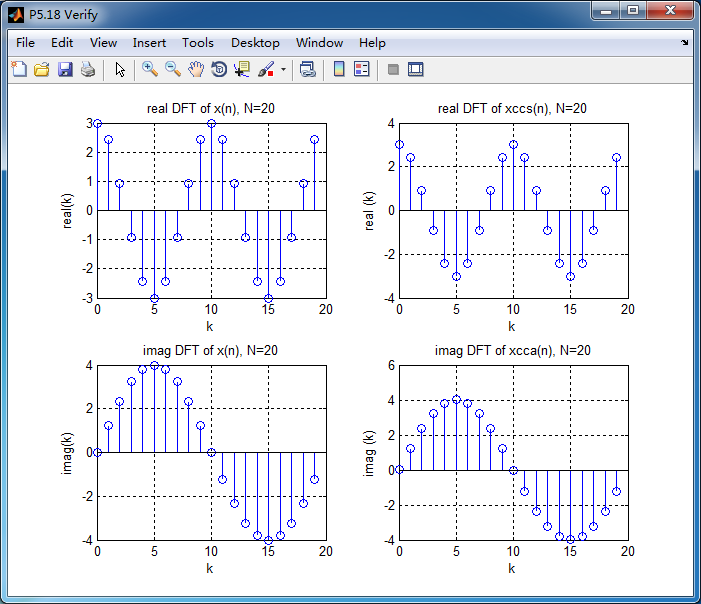
% DFT[xccs] = real(X(k)) DFT[xcca] = j*imag(X(k))
% --------------------------------------------------------------
figure('NumberTitle', 'off', 'Name', 'P5.18 Verify')
set(gcf,'Color','white');
subplot(2,2,1); stem(k1, realXk_DFT);
xlabel('k'); ylabel('real(k)');
title('real DFT of x(n), N=20'); grid on;
subplot(2,2,3); stem(k1, imagXk_DFT);
xlabel('k'); ylabel('imag(k)');
title('imag DFT of x(n), N=20'); grid on;
subplot(2,2,2); stem(k1, realXk_CCS_DFT);
xlabel('k'); ylabel('real (k)');
title('real DFT of xccs(n), N=20'); grid on;
subplot(2,2,4); stem(k1, imagXk_CCA_DFT);
xlabel('k'); ylabel('imag (k)');
title('imag DFT of xcca(n), N=20'); grid on;
error1 = sum( abs(realXk_DFT - realXk_CCS_DFT) )
error2 = sum( abs(imagXk_DFT - imagXk_CCA_DFT) )
% ----------------------------------------------------------------
figure('NumberTitle', 'off', 'Name', 'P5.18 x(n) & xccs(n)')
set(gcf,'Color','white');
subplot(2,2,1); stem(n, real(xn));
xlabel('n'); ylabel('x(n)');
title('real[x(n)], IDFT of X(k)'); grid on;
subplot(2,2,2); stem(n, real(xccs));
xlabel('n'); ylabel('xccs(n)');
title('real xccs'); grid on;
subplot(2,2,3); stem(n, imag(xn));
xlabel('n'); ylabel('x(n)');
title('imag[x(n)], IDFT of X(k)'); grid on;
subplot(2,2,4); stem(n, imag(xccs));
xlabel('n'); ylabel('xccs(n)');
title('imag xccs'); grid on;
% ---------------------------------------------------------------
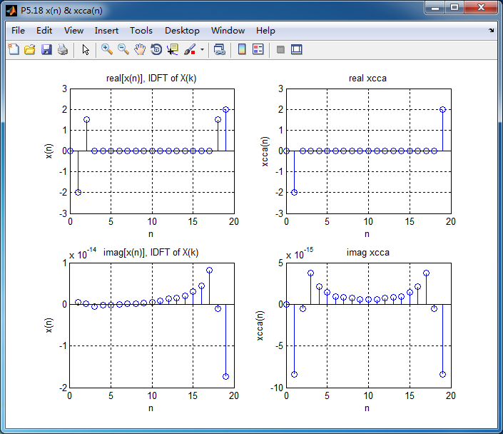
figure('NumberTitle', 'off', 'Name', 'P5.18 x(n) & xcca(n)')
set(gcf,'Color','white');
subplot(2,2,1); stem(n, real(xn));
xlabel('n'); ylabel('x(n)');
title('real[x(n)], IDFT of X(k)'); grid on;
subplot(2,2,2); stem(n, real(xcca));
xlabel('n'); ylabel('xcca(n)');
title('real xcca'); grid on;
subplot(2,2,3); stem(n, imag(xn));
xlabel('n'); ylabel('x(n)');
title('imag[x(n)], IDFT of X(k)'); grid on;
subplot(2,2,4); stem(n, imag(xcca));
xlabel('n'); ylabel('xcca(n)');
title('imag xcca'); grid on;
运行结果:
20点DFT,X(k)
圆周共轭对称序列的DFT

圆周共轭反对称的DFT

从下图看出,序列的DFT X(k)的实部与圆周共轭对称分量的DFT的实部相等;
序列的DFT X(k)的虚部与圆周共轭反对称分量的DFT的虚部相等;
圆周共轭对称序列:xccs(n)

圆周共轭反对称序列xcca(n)