《DSP using MATLAB》示例Example 9.9

代码：

%% ------------------------------------------------------------------------
%%            Output Info about this m-file
fprintf('
***********************************************************
');
fprintf('        <DSP using MATLAB> Exameple 9.9 

');

time_stamp = datestr(now, 31);
[wkd1, wkd2] = weekday(today, 'long');
fprintf('      Now is %20s, and it is %7s  

', time_stamp, wkd2);
%% ------------------------------------------------------------------------

% Given parameters:
I = 5; Rp = 0.1; As = 30; wp = pi/I; ws = pi*0.32; 
[delta1, delta2] = db2delta(Rp, As); weights = [delta2/delta1, 1];
n = [0:50]; x = cos(0.5*pi*n);
n1 = n(1:17); x1 = x(17:33);     % for plotting purposes



%% -----------------------------------------------------------------
%%                             Plot
%% -----------------------------------------------------------------  

% Input signal
Hf1 = figure('units', 'inches', 'position', [1, 1, 8, 6], ...
	'paperunits', 'inches', 'paperposition', [0, 0, 6, 4], ...
	'NumberTitle', 'off', 'Name', 'Exameple 9.9');
set(gcf,'Color','white'); 

TF = 10;

subplot(2, 2, 1); 
Hs1 = stem(n1, x1, 'filled'); set(Hs1, 'markersize', 2, 'color', 'g');
axis([-1, 17, -1.2, 1.2]); grid on;
xlabel('n', 'vertical', 'middle'); ylabel('Amplitude'); 
title('Input Signal x(n)', 'fontsize', TF);
set(gca, 'xtick', [0:4:16]); 
set(gca, 'ytick', [-1, 0, 1]);


% Interpolation with Filter Design: Length M=31
M = 31; F = [0, wp, ws, pi]/pi; A = [I, I, 0, 0];
h = firpm(M-1, F, A, weights); y = upfirdn(x, h, I);
delay = (M-1)/2;           % Delay imparted by the filter
m = delay+1:1:50*I+delay+1; y = y(m); m = 1:81; y = y(81:161);   % for plotting


subplot(2, 2, 2); 
Hs2 = stem(m, y, 'filled'); axis([-5, 85, -1.2, 1.2]); grid on;
xlabel('n', 'vertical', 'middle'); ylabel('Amplitude'); 
title(' Output y(n): I = 5, Filter length=31', 'fontsize', TF);
set(gca, 'xtick', [0:4:16]*I); 
set(gca, 'ytick', [-1, 0, 1]);

% Interpolation with Filter Design: Length M = 51
M = 51; F = [0, wp, ws, pi]/pi; A = [I, I, 0, 0];
h = firpm(M-1, F, A, weights); y = upfirdn(x, h, I);
delay = (M-1)/2;           % Delay imparted by the filter
m = delay+1:1:50*I+delay+1; y = y(m); m = 1:81; y = y(81:161);   % for plotting

subplot(2, 2, 3); 
Hs3 = stem(m, y, 'filled'); axis([-5, 85, -1.2, 1.2]); grid on;
set(Hs3, 'markersize', 2, 'color', 'm');
xlabel('n', 'vertical', 'middle'); ylabel('Amplitude'); 
title('Output y(n): I = 5, Filter length=51 ', 'fontsize', TF);
set(gca, 'xtick', [0:4:16]*I); 
set(gca, 'ytick', [-1, 0, 1]);

% Interpolation with Filter Design : Length M = 81
M = 81; F = [0, wp, ws, pi]/pi; A = [I, I, 0, 0];
h = firpm(M-1, F, A, weights); y = upfirdn(x, h, I);
delay = (M-1)/2;           % Delay imparted by the filter
m = delay+1:1:50*I+delay+1; y = y(m); m = 1:81; y = y(81:161);   % for plotting

subplot(2, 2, 4); 
Hs4 = stem(m, y, 'filled'); axis([-5, 85, -1.2, 1.2]); grid on;
set(Hs4, 'markersize', 2, 'color', 'm');
xlabel('n', 'vertical', 'middle'); ylabel('Amplitude'); 
title('Output y(n): I = 5, Filter length=81 ', 'fontsize', TF);
set(gca, 'xtick', [0:4:16]*I); 
set(gca, 'ytick', [-1, 0, 1]);

　　运行结果：

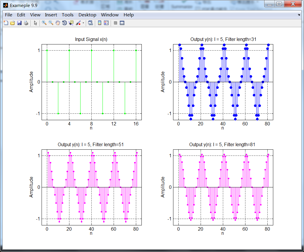
      左上图是输入信号x(n)的一部分，右上图是使用长度为31的滤波器后得到的输出y(n)。对于滤波器延迟和过渡带响应来说，该图是正确的。令人惊讶的是插值后的信号不是其应该的模样。

峰值超过了1，形状有些变形。仔细看图9.20中的滤波器响应表现为宽的过渡带和小的衰减，必然会导致一些谱能量的泄漏，产生变形。

      对于较大的阶数来说，滤波器低通特征较好。信号峰值接近1，并且其形状接近余弦波形。因此，一个好的滤波器设计甚至对一个简单的信号都是严格适用的。