

代码:
M = 20; alpha = (M-1)/2; l = 0:M-1; wl = (2*pi/M)*l;
Hrs = [1, 1, 1, zeros(1, 15), 1, 1]; % Ideal Amp Res sampled
Hdr = [1, 1, 0, 0];
wdl = [0, 0.25, 0.25, 1]; % Ideal Amp Res for plotting
k1 = 0:floor((M-1)/2); k2 = floor((M-1)/2)+1:M-1;
angH = [-alpha*(2*pi)/M*k1, alpha*(2*pi)/M*(M-k2)];
H = Hrs.*exp(j*angH); h = real(ifft(H, M));
[db, mag, pha, grd, w] = freqz_m(h, 1);
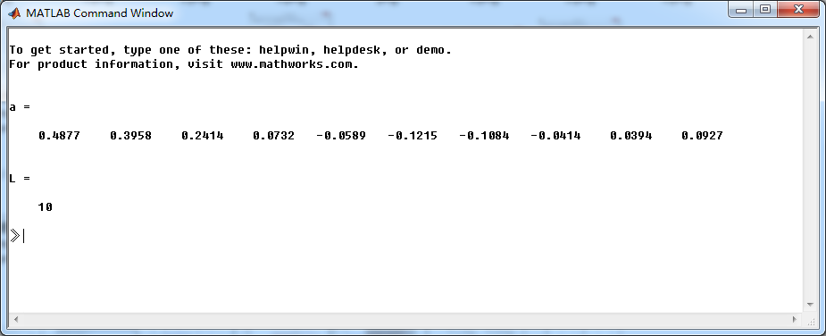
[Hr, ww, a, L] = Hr_Type2(h);
a
L
%Plot
figure('NumberTitle', 'off', 'Name', 'Exameple 7.14')
set(gcf,'Color','white');
subplot(2,2,1); plot(wl(1:11)/pi, Hrs(1:11), 'o', wdl, Hdr); axis([0, 1, -0.1, 1.1]);
xlabel('frequency in pi nuits'); ylabel('Hr(k)'); title('Frequency Samples: M=20');
grid on;
subplot(2,2,2); stem(l, h); axis([-1, M, -0.1, 0.3]);
xlabel('n'); ylabel('h(n)'); title('Impulse Response');
grid on;
subplot(2,2,3); plot(ww/pi, Hr, wl(1:11)/pi, Hrs(1:11), 'o'); axis([0, 1, -0.2, 1.2]); grid on;
xlabel('frequency in pi units'); ylabel('Hr(w)'); title('Amplitude Response');
grid on;
subplot(2,2,4); plot(w/pi, db); axis([0, 1, -60, 10]); grid on;
xlabel('frequency in pi units'); ylabel('Decibels'); title('Magnitude Response');
grid on;
运行结果:
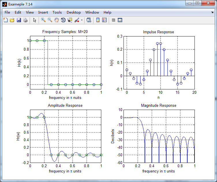
从图上看出,最小的阻带衰减大概16dB,不符要求(50dB)。如果我们增加M的数值,那么
在过渡带中就会出现采样点,其频率响应我们不能精确知晓。所以在实际情况中,我们很少
采用这种naive设计方法。