代码:
%% ------------------------------------------------------------------------
%% Output Info about this m-file
fprintf('
***********************************************************
');
fprintf(' <DSP using MATLAB> Problem 8.28
');
banner();
%% ------------------------------------------------------------------------
Fp = 500; % analog passband freq in Hz
Fs = 700; % analog stopband freq in Hz
fs = 2000; % sampling rate in Hz
% -------------------------------
% ω = ΩT = 2πF/fs
% Digital Filter Specifications:
% -------------------------------
wp = 2*pi*Fp/fs; % digital passband freq in rad/sec
%wp = Fp;
ws = 2*pi*Fs/fs; % digital stopband freq in rad/sec
%ws = Fs;
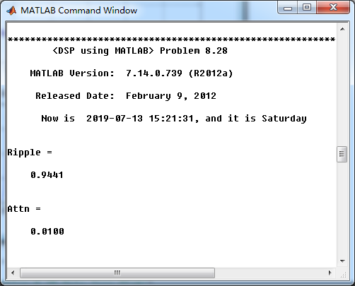
Rp = 0.5; % passband ripple in dB
As = 40; % stopband attenuation in dB
Ripple = 10 ^ (-Rp/20) % passband ripple in absolute
Attn = 10 ^ (-As/20) % stopband attenuation in absolute
% Analog prototype specifications: Inverse Mapping for frequencies
T = 1/fs; % set T = 1
OmegaP = wp/T; % prototype passband freq
OmegaS = ws/T; % prototype stopband freq
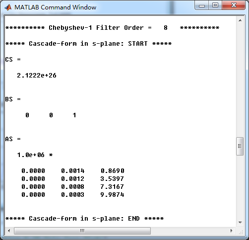
% Analog Chebyshev-1 Prototype Filter Calculation:
[cs, ds] = afd_chb1(OmegaP, OmegaS, Rp, As);
% Calculation of second-order sections:
fprintf('
***** Cascade-form in s-plane: START *****
');
[CS, BS, AS] = sdir2cas(cs, ds)
fprintf('
***** Cascade-form in s-plane: END *****
');
% Calculation of Frequency Response:
[db_s, mag_s, pha_s, ww_s] = freqs_m(cs, ds, 2*pi/T);
% Calculation of Impulse Response:
[ha, x, t] = impulse(cs, ds);
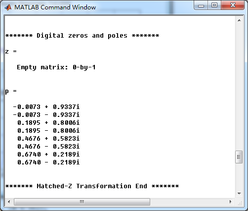
% Match-z Transformation:
%[b, a] = imp_invr(cs, ds, T) % digital Num and Deno coefficients of H(z)
[b, a] = mzt(cs, ds, T) % digital Num and Deno coefficients of H(z)
[C, B, A] = dir2par(b, a)
% Calculation of Frequency Response:
[db, mag, pha, grd, ww] = freqz_m(b, a);
%% -----------------------------------------------------------------
%% Plot
%% -----------------------------------------------------------------
figure('NumberTitle', 'off', 'Name', 'Problem 8.28 Analog Chebyshev-1 lowpass')
set(gcf,'Color','white');
M = 1.2; % Omega max
subplot(2,2,1); plot(ww_s/(pi*1000), mag_s); grid on; axis([-1.5, 1.5, 0, 1.1]);
xlabel(' Analog frequency in kpi units'); ylabel('|H|'); title('Magnitude in Absolute');
set(gca, 'XTickMode', 'manual', 'XTick', [-700, -500, 0, 500, 700, 1000]*0.002);
set(gca, 'YTickMode', 'manual', 'YTick', [0, 0.01, 0.5, 0.9441, 1]);
subplot(2,2,2); plot(ww_s/(pi*1000), db_s); grid on; %axis([0, M, -50, 10]);
xlabel('Analog frequency in kpi units'); ylabel('Decibels'); title('Magnitude in dB ');
set(gca, 'XTickMode', 'manual', 'XTick', [-700, -500, 0, 500, 700, 1000]*0.002);
set(gca, 'YTickMode', 'manual', 'YTick', [-70, -40, -1, 0]);
set(gca,'YTickLabelMode','manual','YTickLabel',['70';'40';' 1';' 0']);
subplot(2,2,3); plot(ww_s/(pi*1000), pha_s/pi); grid on; axis([-1.5, 1.5, -1.2, 1.2]);
xlabel('Analog frequency in kpi nuits'); ylabel('radians'); title('Phase Response');
set(gca, 'XTickMode', 'manual', 'XTick', [-700, -500, 0, 500, 700, 1000]*0.002);
set(gca, 'YTickMode', 'manual', 'YTick', [-1:0.5:1]);
subplot(2,2,4); plot(t, ha); grid on; %axis([0, 30, -0.05, 0.25]);
xlabel('time in seconds'); ylabel('ha(t)'); title('Impulse Response');
figure('NumberTitle', 'off', 'Name', 'Problem 8.28 Digital Chebyshev-1 lowpass')
set(gcf,'Color','white');
M = 2; % Omega max
%% Note %%
%% Magnitude of H(z) * T
%% Note %%
subplot(2,2,1); plot(ww/pi, mag/10); grid on; axis([0, M, 0, 1.1]);
xlabel(' frequency in pi units'); ylabel('|H|'); title('Magnitude Response');
set(gca, 'XTickMode', 'manual', 'XTick', [0, 0.5, 0.7, 1.0, M]);
set(gca, 'YTickMode', 'manual', 'YTick', [0, 0.01, 0.5, 0.9441, 1, 5, 10]);
subplot(2,2,2); plot(ww/pi, pha/pi); axis([0, M, -1.1, 1.1]); grid on;
xlabel('frequency in pi nuits'); ylabel('radians in pi units'); title('Phase Response');
set(gca, 'XTickMode', 'manual', 'XTick', [0, 0.5, 0.7, 1.0, M]);
set(gca, 'YTickMode', 'manual', 'YTick', [-1:1:1]);
subplot(2,2,3); plot(ww/pi, db); axis([0, M, -70, 10]); grid on;
xlabel('frequency in pi units'); ylabel('Decibels'); title('Magnitude in dB ');
set(gca, 'XTickMode', 'manual', 'XTick', [0, 0.5, 0.7, 1.0, M]);
set(gca, 'YTickMode', 'manual', 'YTick', [-50, -40, -1, 0]);
set(gca,'YTickLabelMode','manual','YTickLabel',['50';'40';' 1';' 0']);
subplot(2,2,4); plot(ww/pi, grd); grid on; %axis([0, M, 0, 35]);
xlabel('frequency in pi units'); ylabel('Samples'); title('Group Delay');
set(gca, 'XTickMode', 'manual', 'XTick', [0, 0.5, 0.7, 1.0, M]);
%set(gca, 'YTickMode', 'manual', 'YTick', [0:5:35]);
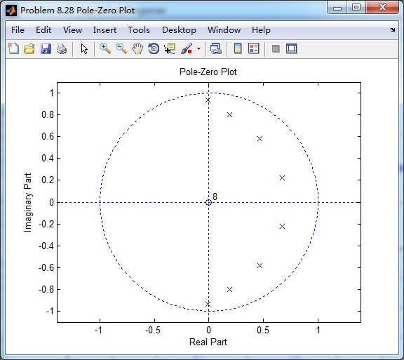
figure('NumberTitle', 'off', 'Name', 'Problem 8.28 Pole-Zero Plot')
set(gcf,'Color','white');
zplane(b,a);
title(sprintf('Pole-Zero Plot'));
%pzplotz(b,a);
% Calculation of Impulse Response:
%[hs, xs, ts] = impulse(c, d);
figure('NumberTitle', 'off', 'Name', 'Problem 8.28 Imp & Freq Response')
set(gcf,'Color','white');
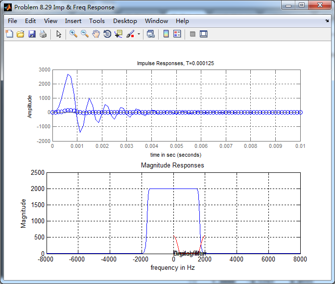
t = [0:0.0005:0.04]; subplot(2,1,1); impulse(cs,ds,t); grid on; % Impulse response of the analog filter
axis([0, 0.04, -500, 1000]);hold on
n = [0:1:0.04/T]; hn = filter(b,a,impseq(0,0,0.04/T)); % Impulse response of the digital filter
stem(n*T,hn); xlabel('time in sec'); title (sprintf('Impulse Responses, T=%.4f',T));
hold off
%n = [0:1:29];
%hz = impz(b, a, n);
% Calculation of Frequency Response:
[dbs, mags, phas, wws] = freqs_m(cs, ds, 2*pi/T); % Analog frequency s-domain
[dbz, magz, phaz, grdz, wwz] = freqz_m(b, a); % Digital z-domain
%% -----------------------------------------------------------------
%% Plot
%% -----------------------------------------------------------------
M = 1/T; % Omega max
subplot(2,1,2); plot(wws/(2*pi),mags*Fs,'b', wwz/(2*pi)*Fs,magz,'r'); grid on;
xlabel('frequency in Hz'); title('Magnitude Responses'); ylabel('Magnitude');
text(1.4,.5,'Analog filter'); text(1.5,1.5,'Digital filter');
运行结果:
转换成绝对指标
模拟Chebyshev-1型低通滤波器,系统函数串联形式
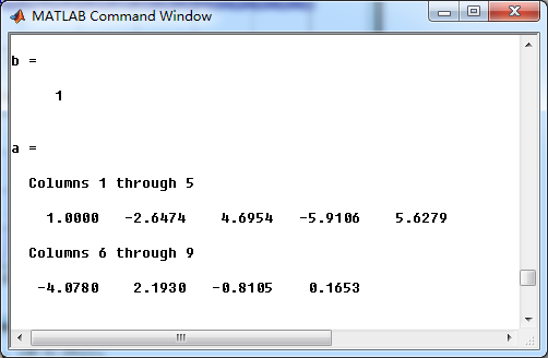
通过match-z方法,模拟低通转换成数字Chebyshev-1型低通滤波器,

数字Chebyshev-1型低通直接形式的系数
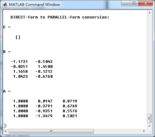
转换成并联形式,其系数
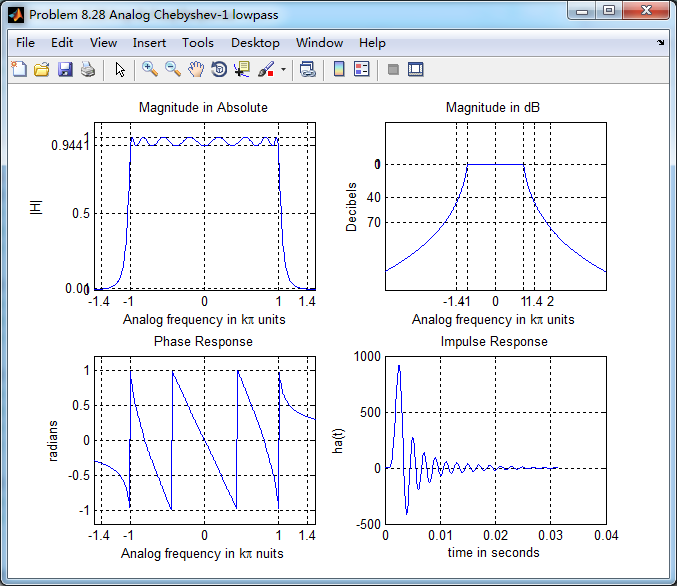
模拟低通的幅度谱、相位谱和脉冲响应
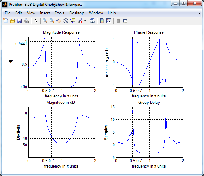
数字低通的幅度谱、相位谱和群延迟
数字低通的零极点图,可以看出,零极点都位于单位圆内。
match-z方法,是和脉冲响应不变法不同的,不保留脉冲响应的形式,模拟Chebyshev-1型低通滤波器和对应的数字低通
滤波器的脉冲响应形式是不同的,见下图。