代码:
%% ++++++++++++++++++++++++++++++++++++++++++++++++++++++++++++++++++++++++++++++++
%% Output Info about this m-file
fprintf('
***********************************************************
');
fprintf(' <DSP using MATLAB> Problem 7.13
');
banner();
%% ++++++++++++++++++++++++++++++++++++++++++++++++++++++++++++++++++++++++++++++++
% bandstop
wp1 = 0.25*pi; ws1 = 0.35*pi; ws2=0.65*pi; wp2=0.75*pi; delta1 = 0.025; delta2 = 0.005;
tr_width = min(ws1-wp1, wp2-ws2);
f = [wp1, ws1, ws2, wp2]/pi;
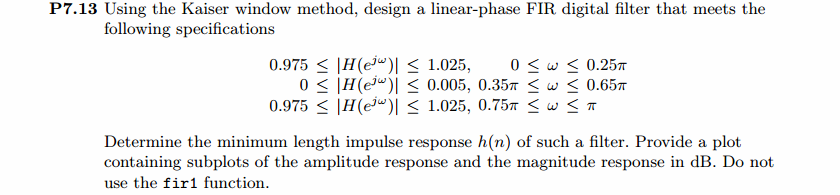
[Rp, As] = delta2db(delta1, delta2)
M = ceil((As-7.95)/(2.285*tr_width)) + 1; % Kaiser Window
if As > 21 || As < 50
beta = 0.5842*(As-21)^0.4 + 0.07886*(As-21);
else
beta = 0.1102*(As-8.7);
end
fprintf('
Kaiser Window method, Filter Length: M = %d. beta = %.4f
', M, beta);
n = [0:1:M-1]; wc1 = (ws1+wp1)/2; wc2 = (ws2+wp2)/2;
%wc = (ws + wp)/2, % ideal LPF cutoff frequency
hd = ideal_lp(wc1, M) + ideal_lp(pi, M) - ideal_lp(wc2, M);
w_kai = (kaiser(M, beta))'; h = hd .* w_kai;
[db, mag, pha, grd, w] = freqz_m(h, [1]); delta_w = 2*pi/1000;
[Hr,ww,P,L] = ampl_res(h);
Rp = -(min(db(1 :1: floor(wp1/delta_w)+1))); % Actual Passband Ripple
fprintf('
Actual Passband Ripple is %.4f dB.
', Rp);
As = -round(max(db(ws1/delta_w+1 : 1 : ws2/delta_w ))); % Min Stopband attenuation
fprintf('
Min Stopband attenuation is %.4f dB.
', As);
[delta1, delta2] = db2delta(Rp, As)
%% ----------------------------------
%% Increse M
%% ----------------------------------
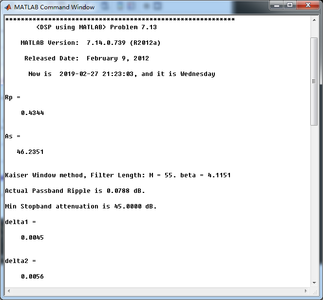
M = M+2
hd = ideal_lp(wc1, M) + ideal_lp(pi, M) - ideal_lp(wc2, M);
w_kai = (kaiser(M, beta))'; h = hd .* w_kai;
[db, mag, pha, grd, w] = freqz_m(h, [1]); delta_w = 2*pi/1000;
[Hr,ww,P,L] = ampl_res(h);
Rp = -(min(db(1 :1: floor(wp1/delta_w)+1))); % Actual Passband Ripple
fprintf('
Actual Passband Ripple is %.4f dB.
', Rp);
As = -round(max(db(ws1/delta_w+1 : 1 : ws2/delta_w ))); % Min Stopband attenuation
fprintf('
Min Stopband attenuation is %.4f dB.
', As);
[delta1, delta2] = db2delta(Rp, As)
n = [0:1:M-1];
% Plot
figure('NumberTitle', 'off', 'Name', 'Problem 7.13 ideal_lp Method')
set(gcf,'Color','white');
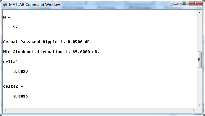
subplot(2,2,1); stem(n, hd); axis([0 M-1 -0.2 0.6]); grid on;
xlabel('n'); ylabel('hd(n)'); title('Ideal Impulse Response');
subplot(2,2,2); stem(n, w_kai); axis([0 M-1 0 1.1]); grid on;
xlabel('n'); ylabel('w(n)'); title('Kaiser Window');
subplot(2,2,3); stem(n, h); axis([0 M-1 -0.2 0.6]); grid on;
xlabel('n'); ylabel('h(n)'); title('Actual Impulse Response');
subplot(2,2,4); plot(w/pi, db); axis([0 1 -100 10]); grid on;
set(gca,'YTickMode','manual','YTick',[-90,-49,0]);
set(gca,'YTickLabelMode','manual','YTickLabel',['90';'49';' 0']);
set(gca,'XTickMode','manual','XTick',[0,f,1]);
xlabel('frequency in pi units'); ylabel('Decibels'); title('Magnitude Response in dB');
figure('NumberTitle', 'off', 'Name', 'Problem 7.13 h(n) ideal_lp Method')
set(gcf,'Color','white');
subplot(2,2,1); plot(w/pi, db); grid on; axis([0 2 -100 10]);
xlabel('frequency in pi units'); ylabel('Decibels'); title('Magnitude Response in dB');
set(gca,'YTickMode','manual','YTick',[-90,-49,0])
set(gca,'YTickLabelMode','manual','YTickLabel',['90';'49';' 0']);
set(gca,'XTickMode','manual','XTick',[0,f,1+f,2]);
subplot(2,2,3); plot(w/pi, mag); grid on; %axis([0 2 -100 10]);
xlabel('frequency in pi units'); ylabel('Absolute'); title('Magnitude Response in absolute');
set(gca,'XTickMode','manual','XTick',[0,f,1+f,2]);
set(gca,'YTickMode','manual','YTick',[0.0,0.5,1.0])
subplot(2,2,2); plot(w/pi, pha); grid on; %axis([0 1 -100 10]);
xlabel('frequency in pi units'); ylabel('Rad'); title('Phase Response in Radians');
subplot(2,2,4); plot(w/pi, grd*pi/180); grid on; %axis([0 1 -100 10]);
xlabel('frequency in pi units'); ylabel('Rad'); title('Group Delay');
figure('NumberTitle', 'off', 'Name', 'Problem 7.13 h(n)')
set(gcf,'Color','white');
plot(ww/pi, Hr); grid on; %axis([0 1 -100 10]);
xlabel('frequency in pi units'); ylabel('Hr'); title('Amplitude Response');
set(gca,'YTickMode','manual','YTick',[-delta2,0,delta2,1 - delta1,1, 1 + delta1])
%set(gca,'YTickLabelMode','manual','YTickLabel',['90';'45';' 0']);
set(gca,'XTickMode','manual','XTick',[0,f,2]);
%% +++++++++++++++++++++++++++++++++++++++++
%% fir1 function method
%% +++++++++++++++++++++++++++++++++++++++++
f = [wp1, ws1, ws2, wp2]/pi;
m = [1 0 1];
ripple = [0.025 0.005 0.025];
[N, wc, beta, ftype] = kaiserord(f,m,ripple);
fprintf('
------------ kaiserord function: START---------------
');
fprintf('
--------- results used by fir1 function ---------
');
N
wc
beta
ftype
fprintf('------------- kaiserord function: FINISH---------------
');
%h_check = fir1(M-1, [wc1 wc2]/pi, 'stop', window(@kaiser, M));
%h_check = fir1(N, wc, ftype, window(@kaiser, N+1));
h_check = fir1(N, wc, ftype, kaiser(N+1, beta));
[db, mag, pha, grd, w] = freqz_m(h_check, [1]);
[Hr,ww,P,L] = ampl_res(h_check);
Rp = -(min(db(1 :1: floor(wp1/delta_w)+1))); % Actual Passband Ripple
fprintf('
Actual Passband Ripple is %.4f dB.
', Rp);
As = -round(max(db(ws1/delta_w+1 : 1 : ws2/delta_w ))); % Min Stopband attenuation
fprintf('
Min Stopband attenuation is %.4f dB.
', As);
%% ----------------------------------
%% Increse N
%% ----------------------------------
N = N+2
h_check = fir1(N, wc, ftype, kaiser(N+1, beta));
[db, mag, pha, grd, w] = freqz_m(h_check, [1]);
[Hr,ww,P,L] = ampl_res(h_check);
As = -round(max(db(ws1/delta_w+1 : 1 : ws2/delta_w ))); % Min Stopband attenuation
fprintf('
Min Stopband attenuation is %.4f dB.
', As);
figure('NumberTitle', 'off', 'Name', 'Problem 7.13 fir1 Method')
set(gcf,'Color','white');
subplot(2,2,1); stem(n, hd); axis([0 M-1 -0.2 0.6]); grid on;
xlabel('n'); ylabel('hd(n)'); title('Ideal Impulse Response');
subplot(2,2,2); stem(n, w_kai); axis([0 M-1 0 1.1]); grid on;
xlabel('n'); ylabel('w(n)'); title('Kaiser Window');
subplot(2,2,3); stem([0:N], h_check); axis([0 M -0.2 0.7]); grid on;
xlabel('n'); ylabel('h\_check(n)'); title('Actual Impulse Response');
subplot(2,2,4); plot(w/pi, db); axis([0 1 -100 10]); grid on;
set(gca,'YTickMode','manual','YTick',[-90,-49,0])
set(gca,'YTickLabelMode','manual','YTickLabel',['90';'49';' 0']);
set(gca,'XTickMode','manual','XTick',[0,f,1]);
xlabel('frequency in pi units'); ylabel('Decibels'); title('Magnitude Response in dB');
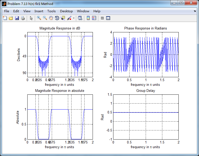
figure('NumberTitle', 'off', 'Name', 'Problem 7.13 h(n) fir1 Method')
set(gcf,'Color','white');
subplot(2,2,1); plot(w/pi, db); grid on; axis([0 2 -100 10]);
xlabel('frequency in pi units'); ylabel('Decibels'); title('Magnitude Response in dB');
set(gca,'YTickMode','manual','YTick',[-90,-49,0])
set(gca,'YTickLabelMode','manual','YTickLabel',['90';'49';' 0']);
set(gca,'XTickMode','manual','XTick',[0,f,1+f,2]);
subplot(2,2,3); plot(w/pi, mag); grid on; %axis([0 1 -100 10]);
xlabel('frequency in pi units'); ylabel('Absolute'); title('Magnitude Response in absolute');
set(gca,'XTickMode','manual','XTick',[0,f,1+f,2]);
set(gca,'YTickMode','manual','YTick',[0.0,0.5,1.0])
subplot(2,2,2); plot(w/pi, pha); grid on; %axis([0 1 -100 10]);
xlabel('frequency in pi units'); ylabel('Rad'); title('Phase Response in Radians');
subplot(2,2,4); plot(w/pi, grd*pi/180); grid on; %axis([0 1 -100 10]);
xlabel('frequency in pi units'); ylabel('Rad'); title('Group Delay');
运行结果:
最小阻带衰减设计是46.2351dB,kaiser窗长度M=57时满足要求。
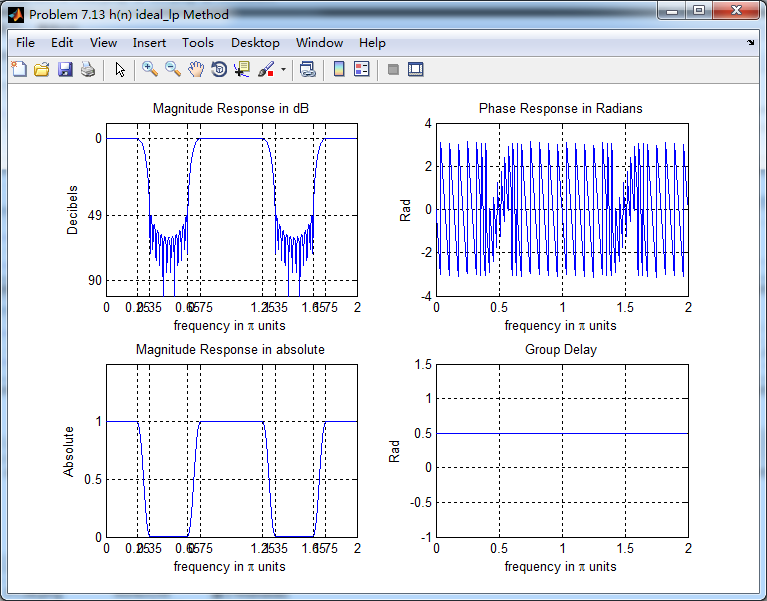
利用Kaiser窗得到的脉冲响应,计算其幅度响应(dB和Absolute单位)、相位响应和群延迟响应。
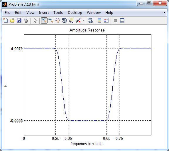
振幅响应
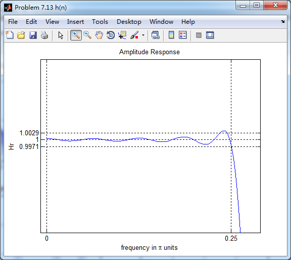
通带部分
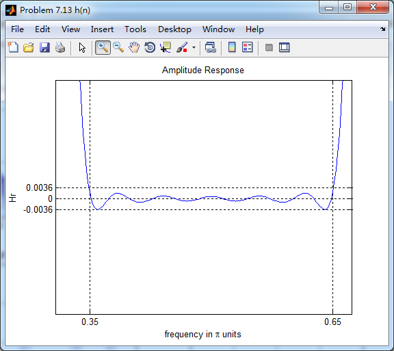
阻带部分
利用fir1函数得到脉冲响应,和前面进行对比


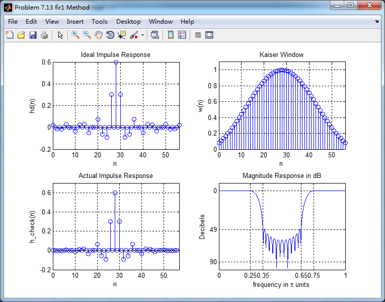
两种方法,区别不大。