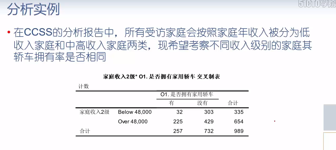


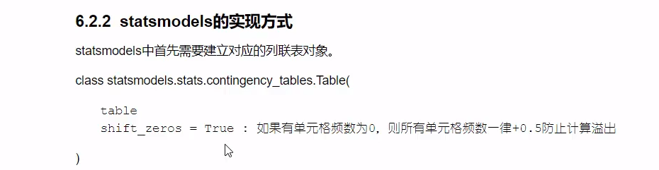
import statsmodels.stats.contingency_tables as tb  # 卡方检验,不同家庭收入级别在轿车拥有率上是否有区别
table = tb.Table(pd.crosstab(ccss.Ts9, ccss.O1))
table
<statsmodels.stats.contingency_tables.Table at 0x1df819bc5c0>
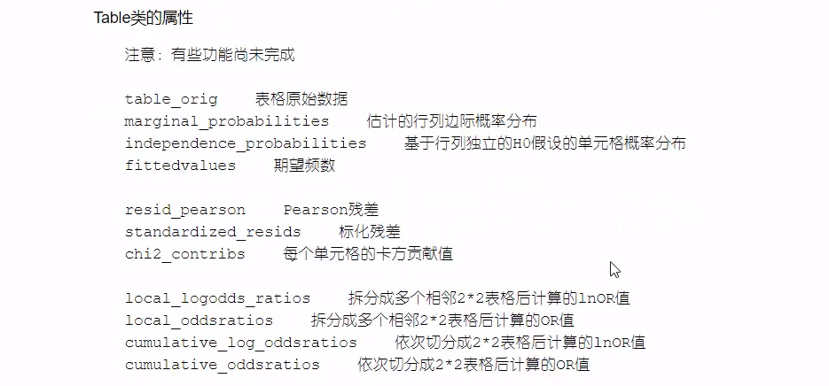
table.table_orig
| O1 | 有 | 没有 |
|---|---|---|
| Ts9 | ||
| Below 48,000 | 32 | 303 |
| Over 48,000 | 225 | 429 |
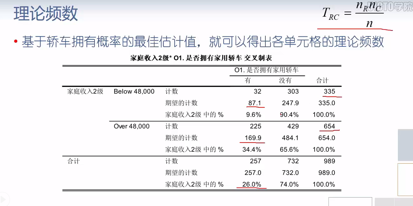
table.fittedvalues
| O1 | 有 | 没有 |
|---|---|---|
| Ts9 | ||
| Below 48,000 | 87.052578 | 247.947422 |
| Over 48,000 | 169.947422 | 484.052578 |
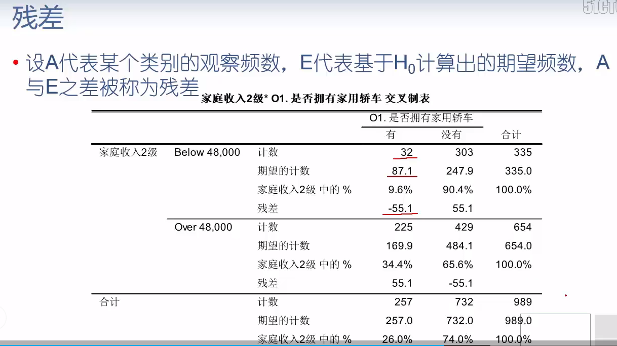
table.resid_pearson
| O1 | 有 | 没有 |
|---|---|---|
| Ts9 | ||
| Below 48,000 | -5.900473 | 3.496213 |
| Over 48,000 | 4.222993 | -2.502254 |
table.chi2_contribs
| O1 | 有 | 没有 |
|---|---|---|
| Ts9 | ||
| Below 48,000 | 34.815584 | 12.223504 |
| Over 48,000 | 17.833671 | 6.261275 |
table.marginal_probabilities
(Ts9
 Below 48,000    0.338726
 Over 48,000     0.661274
 dtype: float64, O1
 有     0.259858
 没有    0.740142
 dtype: float64)
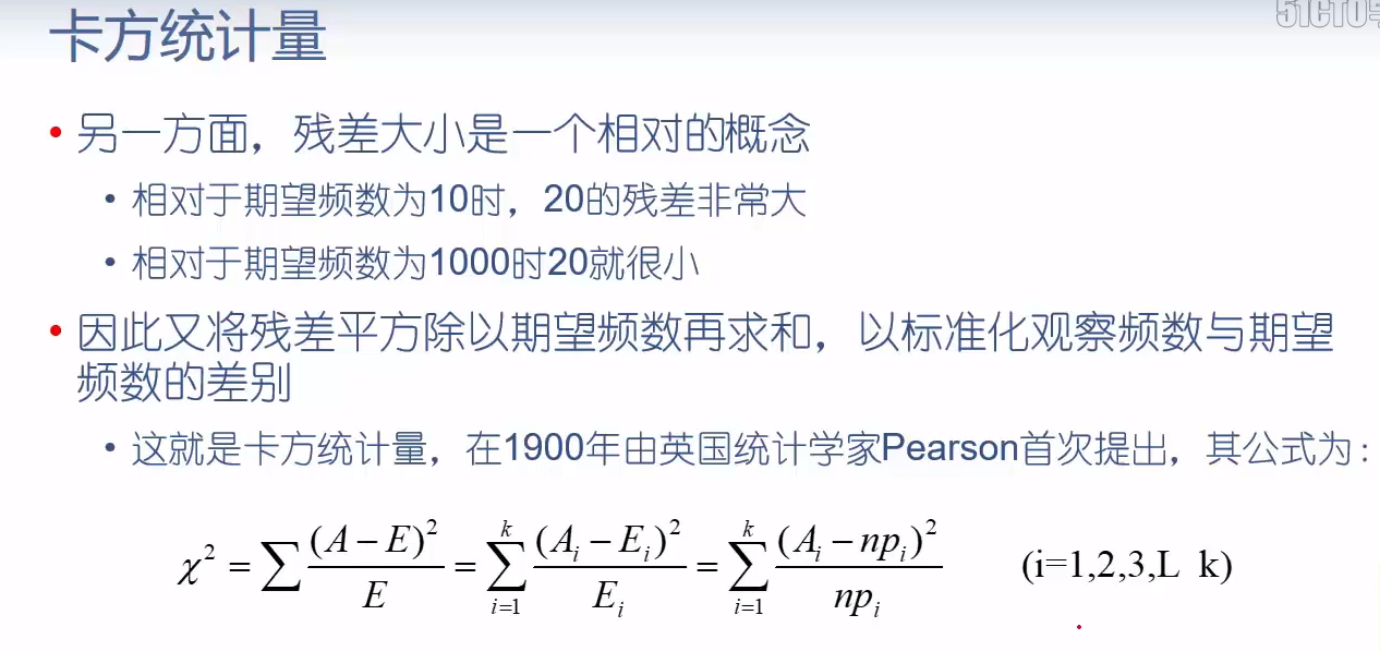
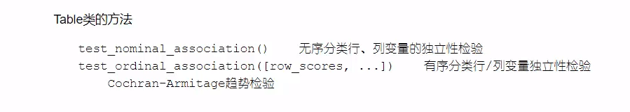
res = table.test_nominal_association()
res.statistic # 卡方统计量
71.13403472094657
res.df # 自由度
1
res.pvalue # p值
0.0
# 不同城市的轿车拥有比率是否相同
table2 = tb.Table(pd.crosstab(ccss.s0, ccss.O1))
table2.table_orig
| O1 | 有 | 没有 |
|---|---|---|
| s0 | ||
| 上海 | 87 | 300 |
| 北京 | 118 | 258 |
| 广州 | 107 | 274 |
res2 = table2.test_nominal_association()
print(res2.statistic, res2.df, res2.pvalue)  # 拒绝了原假设不同城市轿车拥有比率无差异的情况
7.80961277431242 2 0.02014485441628988
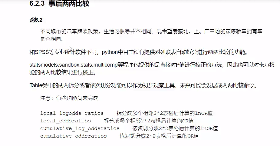
table2.local_oddsratios
| O1 | 有 | 没有 |
|---|---|---|
| s0 | ||
| 上海 | 0.634068 | NaN |
| 北京 | 1.171195 | NaN |
| 广州 | NaN | NaN |
table2.cumulative_oddsratios
| O1 | 有 | 没有 |
|---|---|---|
| s0 | ||
| 上海 | 0.685689 | NaN |
| 北京 | 0.940776 | NaN |
| 广州 | NaN | NaN |

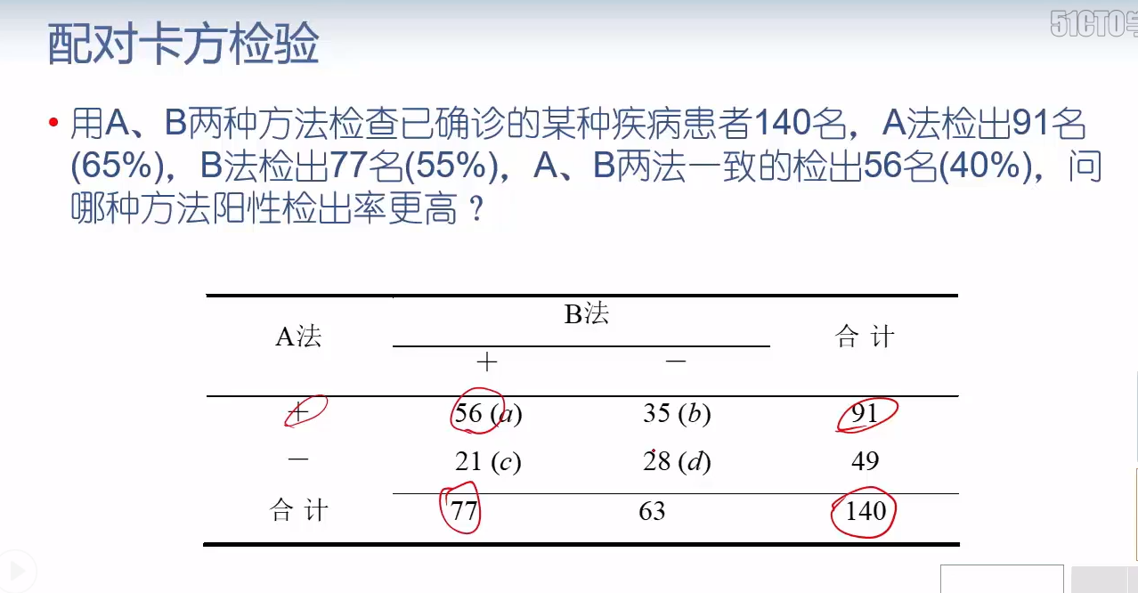
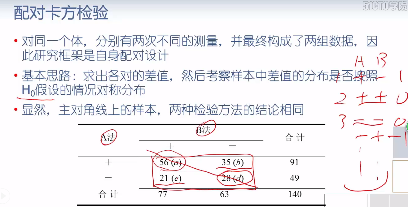
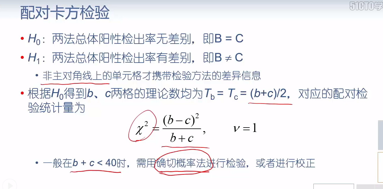

# 配对卡方检验
import statsmodels.stats.contingency_tables as tbl
table3 = tbl.mcnemar(pd.DataFrame([[56, 35], [21, 28]]))
table3.pvalue
0.08142681460950622
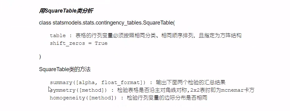
tbl.SquareTable(pd.DataFrame([[5, 35], [21, 2]])).summary()
| Statistic | P-value | DF | |
|---|---|---|---|
| Symmetry | 3.500 | 0.061 | 1 |
| Homogeneity | 3.500 | 0.061 | 1 |
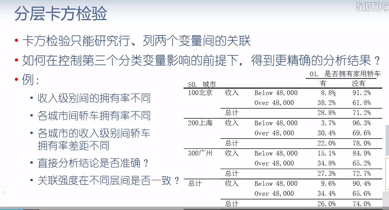

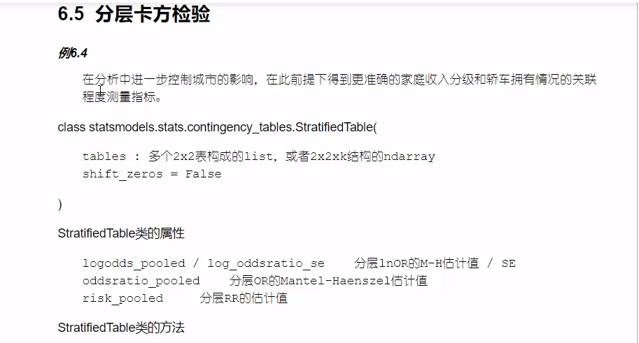
# 分层卡方检验
rawtb = pd.crosstab([ccss.s0, ccss.Ts9], ccss.O1)
rawtb
| O1 | 有 | 没有 | |
|---|---|---|---|
| s0 | Ts9 | ||
| 上海 | Below 48,000 | 4 | 103 |
| Over 48,000 | 70 | 160 | |
| 北京 | Below 48,000 | 9 | 93 |
| Over 48,000 | 83 | 134 | |
| 广州 | Below 48,000 | 19 | 107 |
| Over 48,000 | 72 | 135 |
pd.crosstab([ccss.s0, ccss.Ts9], ccss.O1, normalize=0)
| O1 | 有 | 没有 | |
|---|---|---|---|
| s0 | Ts9 | ||
| 上海 | Below 48,000 | 0.037383 | 0.962617 |
| Over 48,000 | 0.304348 | 0.695652 | |
| 北京 | Below 48,000 | 0.088235 | 0.911765 |
| Over 48,000 | 0.382488 | 0.617512 | |
| 广州 | Below 48,000 | 0.150794 | 0.849206 |
| Over 48,000 | 0.347826 | 0.652174 |
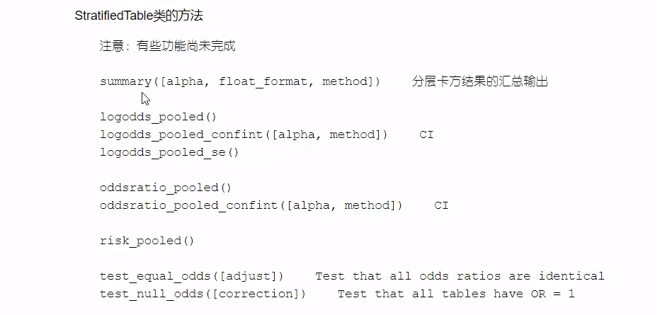
table4 = tbl.StratifiedTable([rawtb[:2],
                             rawtb[2:4],
                             rawtb[4:]]
                            )
table4.summary()  # Test constant OR先查看层和层之间的关联强度是否是不变的,如果不同,不能进行合并,这边显然p值拒绝了关联强度相同的结论,如果关联结论相同则再看Test of OR行列变量有无关联
| Estimate | LCB | UCB | |
|---|---|---|---|
| Pooled odds | 0.195 | 0.130 | 0.292 |
| Pooled log odds | -1.636 | -2.040 | -1.232 |
| Pooled risk ratio | 0.272 | ||
| Statistic | P-value | ||
| Test of OR=1 | 72.178 | 0.000 | |
| Test constant OR | 6.165 | 0.046 | |
| Number of tables | 3 | ||
| Min n | 319 | ||
| Max n | 337 | ||
| Avg n | 330 | ||
| Total n | 989 |


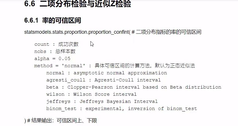

from statsmodels.stats import proportion as sp
sp.proportion_confint(5, 10)  # 使用近似正态计算95%置信区间
(0.19010248384771916, 0.8098975161522808)
sp.proportion_confint(5, 10, method='binom_test') # 使用精确计算概率值
(0.2224411010081248, 0.7775588989918751)
sp.multinomial_proportions_confint([5, 5])
array([[0.21086627, 0.78913373],
       [0.21086627, 0.78913373]])
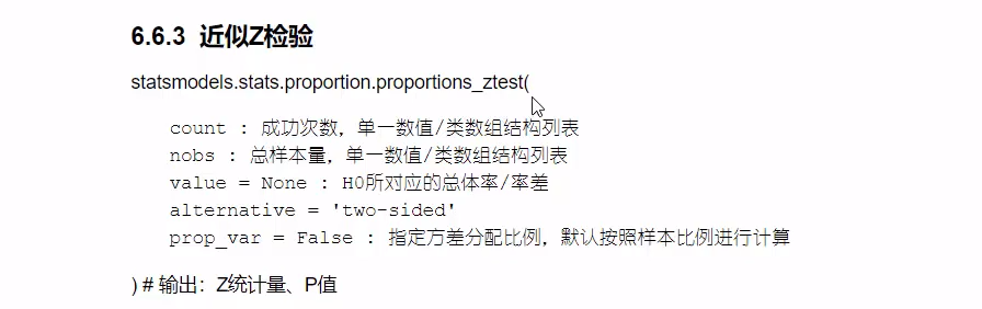
sp.proportions_ztest(30, 100, 0.2) # 总次数100,成功30次,是否偏离总体率0.2
(2.182178902359923, 0.029096331741252257)
sp.proportions_ztest([30, 25], [100, 200], 0) # a组100例成功30例,b组200例成功25例,0是指定的两总体率的差异
(3.692744729379982, 0.00022184668066321168)