library(readxl)
library(TSA)
library(fUnitRoots)
library(fBasics)
library(tseries)
library(forecast)
library(urca)

# 导入数据
xlsx_1<-read_excel("~/Desktop/graduation design/WIND/export for USA.xlsx",
                   sheet = "Sheet2")
# 提取数据,300个数据
mon <- xlsx_1[,2]

# 构建时间序列
mon.timeseries <- ts(mon,start = c(1995,1),end = c(2019,12),frequency = 12)
difflogmon = diff(log(mon.timeseries))
根据时序图可以看到出口序列具有很强的季节性和增长趋势
为了将其变为平稳数据,并且消除趋势,对出口数据取对数差分,得到收益率(增长率)序列
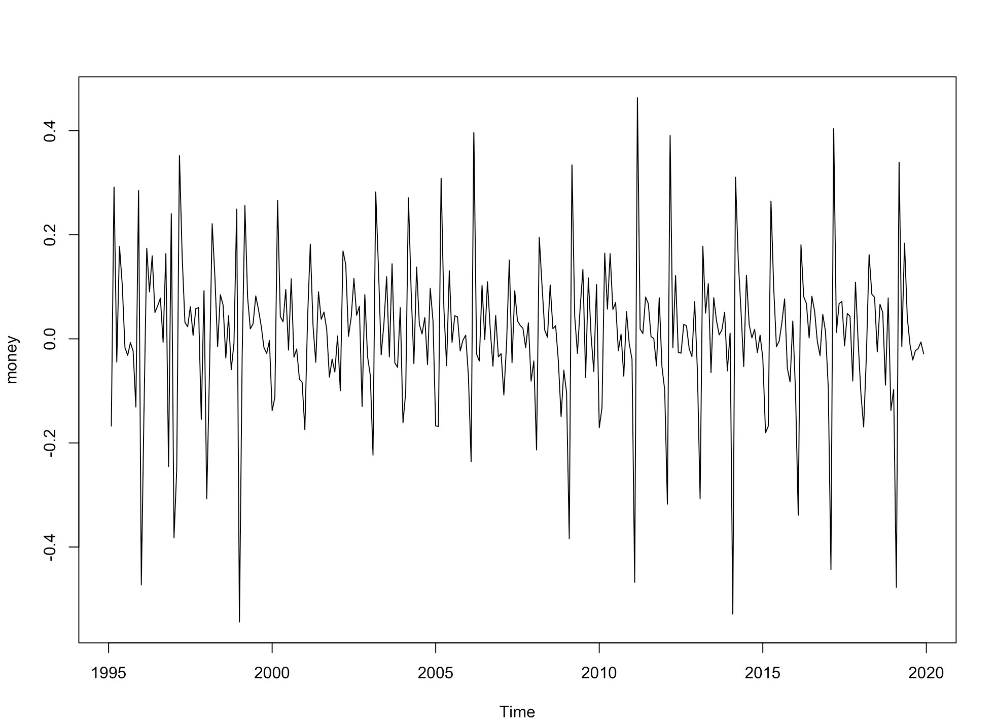
根据上图初步判定收益率为平稳序列
为了能进行变点检验,选取1995-2000的数据建立模型
下面首先进行平稳性检验
mon1.timeseries <- ts(mon,start = c(1995,1),end = c(2000,12),frequency = 12)

difflogmon1 = diff(log(mon1.timeseries))
df = ur.df(difflogmon1)

summary(df)

###############################################
# Augmented Dickey-Fuller Test Unit Root Test #
###############################################

Test regression none


Call:
lm(formula = z.diff ~ z.lag.1 - 1 + z.diff.lag)

Residuals:
     Min       1Q   Median       3Q      Max
-0.49342 -0.02738  0.04970  0.10349  0.25371

Coefficients:
           Estimate Std. Error t value Pr(>|t|)
z.lag.1     -1.3776     0.1829  -7.530 1.69e-10 ***
z.diff.lag   0.1696     0.1176   1.442    0.154
---
Signif. codes:  0 ‘***’ 0.001 ‘**’ 0.01 ‘*’ 0.05 ‘.’ 0.1 ‘ ’ 1

Residual standard error: 0.1579 on 67 degrees of freedom
Multiple R-squared:  0.6096,    Adjusted R-squared:  0.5979
F-statistic:  52.3 on 2 and 67 DF,  p-value: 2.072e-14


Value of test-statistic is: -7.53

Critical values for test statistics:
     1pct  5pct 10pct
tau1 -2.6 -1.95 -1.61
可见收益率序列是平稳的。
作acf与pacf图
acf(as.vector(difflogmon1),lag.max = 36)
pacf(as.vector(difflogmon1),lag.max = 36)
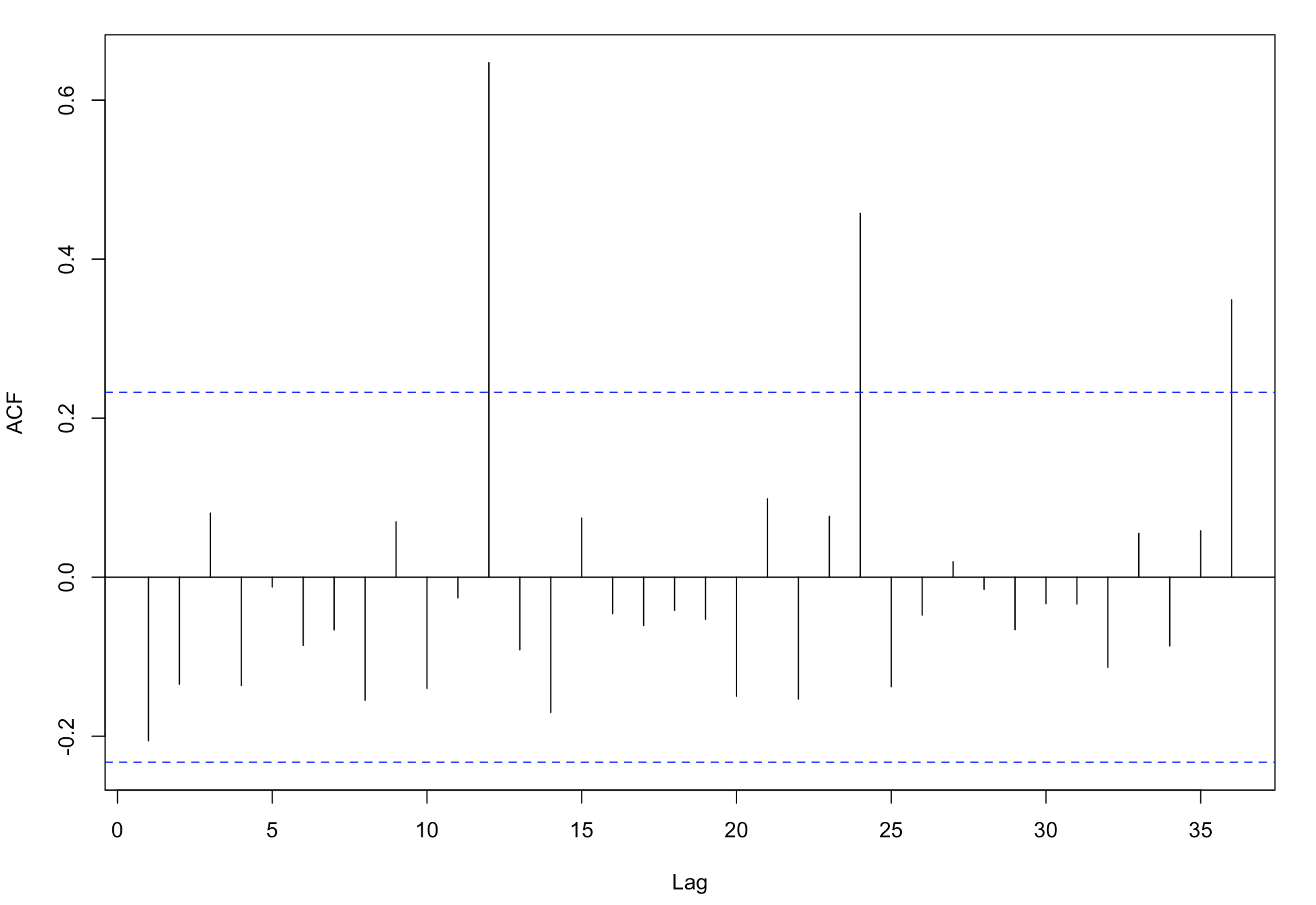
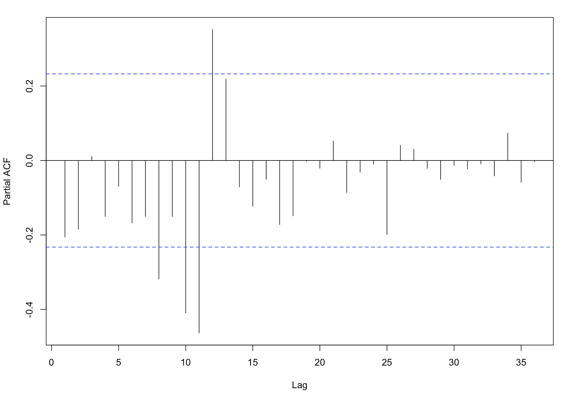
从自相关图来看,数据具有非常强的季节性,并且周期 s = 12。
为了消除季节性,对收益率进行滞后12的一阶差分,观察acf与pacf

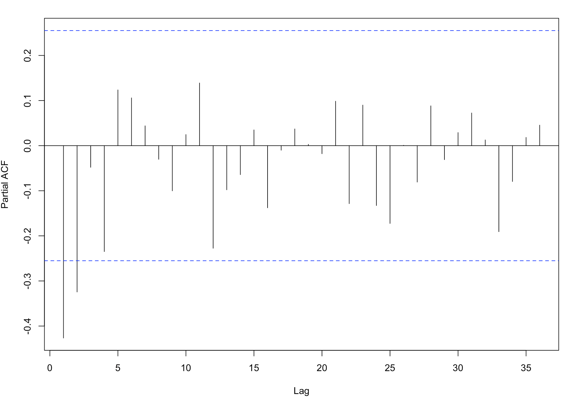
从图中可以看出acf,pacf滞后一阶之后截尾,所以去除季节性的模型应为ARMA(1,1)模型
下面建立季节ARMA模型,消除季节性,利用最大似然法确定参数。
设yt为收益率,根据季节性的特征可能出现在AR或MA中,可能的模型有
![]()
![]()
下面进行参数估计,和利用AIC准则选择最合适的模型
arima(difflogmon1,order = c(1,0,1),seasonal = c(0,1,1))

Call:
arima(x = difflogmon1, order = c(1, 0, 1), seasonal = c(0, 1, 1))

Coefficients:
          ar1      ma1     sma1
      -0.0366  -0.5681  -0.4999
s.e.   0.2176   0.1799   0.1602

sigma^2 estimated as 0.006972:  log likelihood = 60.83,  aic = -115.67


arima(difflogmon1,order = c(1,0,1),seasonal = c(1,1,0))

Call:
arima(x = difflogmon1, order = c(1, 0, 1), seasonal = c(1, 1, 0))

Coefficients:
          ar1      ma1     sar1
      -0.0333  -0.5642  -0.3632
s.e.   0.2137   0.1738   0.1345

sigma^2 estimated as 0.007496:  log likelihood = 59.58,  aic = -113.15
因此选择第二个模型,即建立ARMA(1,0,1)(0,1,1)模型
检验模型
正态性
1.Q-Q图
ar = arima(difflogmon1,order = c(1,0,1),seasonal = c(0,1,1))

qqnorm(ar$residuals)
qqline(ar$residuals)
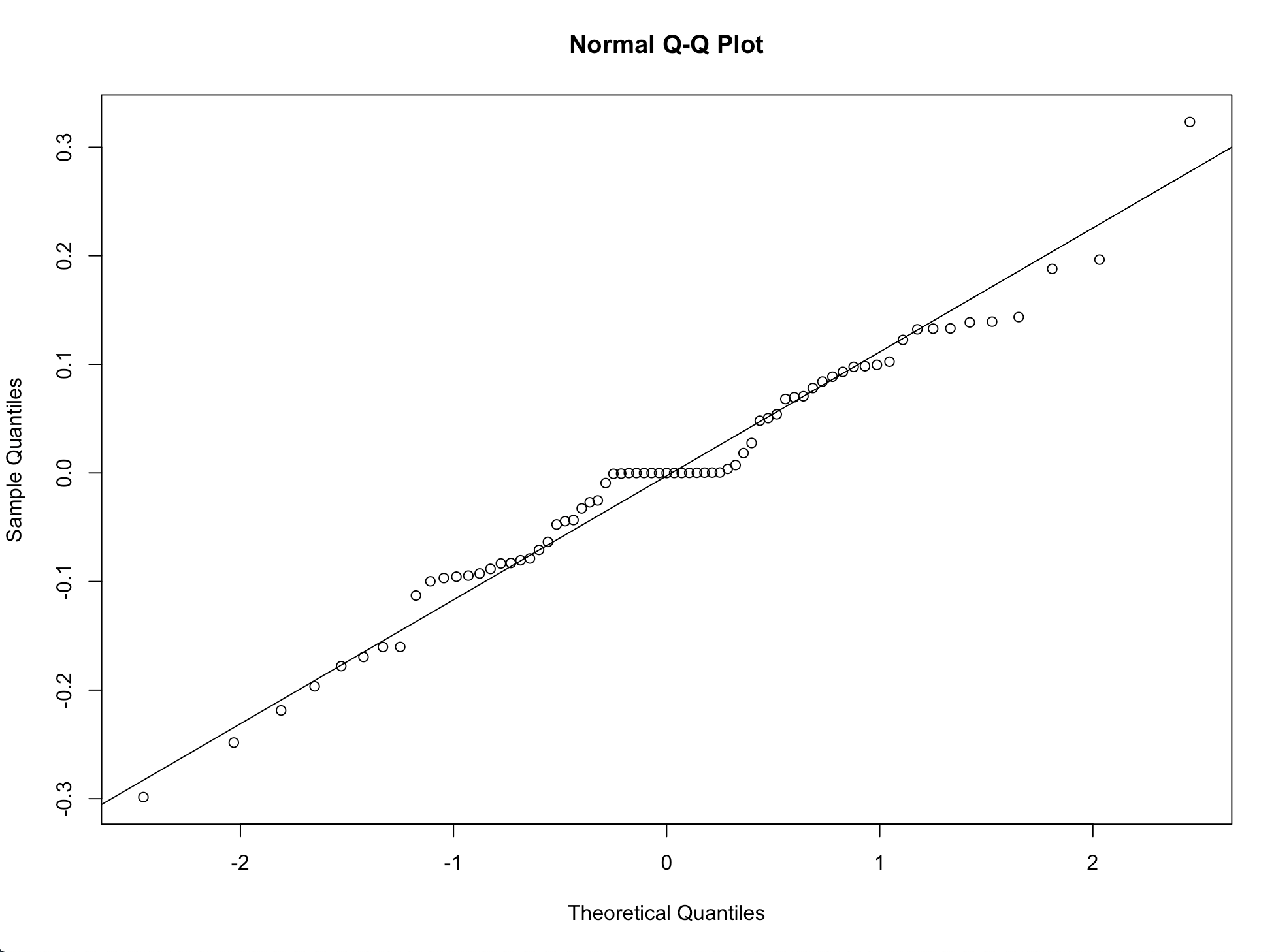
可见模型残差分布在对角线上,符合正态性
2.Shapiro-Wilks检验
shapiro.test(ar$residuals)


    Shapiro-Wilk normality test

data:  ar$residuals
W = 0.98135, p-value = 0.3725
p值大于0.05,接受正态性检验
独立性
根据Box-Pierce和Ljung-Box的Q统计量检验模型的残差是否为白噪声
ar = arima(difflogmon1,order = c(1,0,1),seasonal = c(0,1,1))


Box.test(ar$residuals)

    Box-Pierce test

data:  ar$residuals
X-squared = 0.039468, df = 1, p-value = 0.8425
结果接受白噪声的原假设,因此模型建立。
下面的工作是,利用CUSUM构建统计量,检测2001-2019年的变点位置