Convolution Fundamental I
Foundations of CNNs
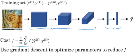
Learning to implement the foundational layers of CNN's (pooling,convolutions) and to stack them properly in a deep network to solve multi-class image classification problems.
Computer vision
Computer vision is from the applications that are rapidly active thanks to deep learning
One of the applications of computer vision that are using deep learning includes:
Self driving cars
Face recognition
Deep learning also is making new arts to be created to in computer vision as we will see.
Rabid changes to computer vison are making new applications that weren't possible a few years ago.
Computer vison deep leraning techniques are always evolving making a new architectures which can help us in other areas other than computer vision
For example, Andrew Ng took some ideas of computer vision and applied it in speech recognition
Examples of a computer vision problems includes:
Image classification
Object detection
Detect object and localize them
Neural style transfer
Changes the style of an image using another image.
On of the challenges of computer vision problem that images can be so large and we want a fast and accurate algorithm to work with that.
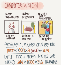
For example,a 1000*1000 image will represent 3 million feature/input to the full connected neural network. If the following hidden layer contains 1000, Then we we will want to learn weight of the shape [1000,3 million] which is 3 billion parameter only in the first layer and that's so computationally expensive!
On of the solutions is to build this using convolution layers instead of the fully connected layers.
Edge detection example
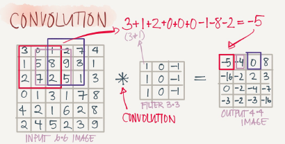
The convolution operation is one of the fundamentals blocks of a CNN. One of the examples about convolution is the image edge detection operation.
Early layers of CNN might detect edges then the middle layers will detect parts of objects and the layers will put the these parts together to produce an output
In an image we can detect vertical edges, horizontal edges,or full edge detector
Vertical edge detection
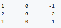
An example of convolution operation to detect vertical edges:
In the last exmple a 6*6 matrix convolved with 3*3 filter/kernel gives us a 4*4 matrix
If you make the convolution operation in TensorFlow you will fin the function tf.nn.conv2d. In keras you will fin conv2d function.
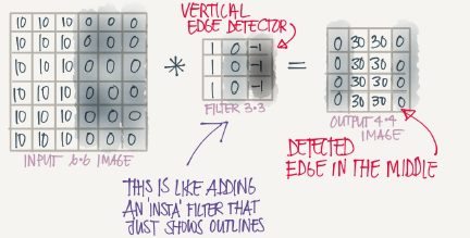
The vertical edge detection filter will find a 3*3 place in an image where there are a bright region followed by a dark region
If we applied this filter to a white region followed by a dark region,it should find the edges in between the two colors as a positive value. But if we applied the same filter to a dark region followed by a white region it will give us negative values. To solve this we can use the abs function to make it positive.
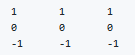
Horizontal edge detection
Filter would be like this
There are a lot of ways we can put number inside the horizontal of vertical edge detections. For example here are the vertical Sobel filter(The idea is taking care of the middle row)
Also something called Scharr filter(The idea is taking great care of the middle row)
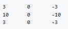
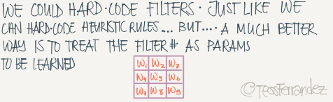
What we learned in the deep learning is that we don't need to hand craft these numbers, we can treat them as weights and then learn them. It can learn horizontal, vertical ,angled, or any edge type automatically ranther than getting them by hand.
Padding
In order to use deep neural networks we really need to use paddings
In the last section we saw that a 6*6 matrix convolved with 3*3 filter/kernel gives us a 4*4 matrix.
To give it a general rule, if a matrix n*n is convolved with f*f filter/kernel give us n-f+1,n-f+1 matrix.
The convolution operation shrinks the matrix if f>1
We want to apply convolution operation multiple times, but if the image shrinks we will lose a lot of data on this process. Also the edges pixels are uses less than other pixels in an image.
So the problems with convolutions are:
shrinks output
throwing away a lot of information that are in the edges.
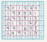
To solve these problems we can pad the input image before convolution by adding some rows and columns to it. We will call the padding amount p the number of row/columns that we will insert in top, bottom , left and right of the image.
In almost all the cases the padding values are zeros
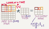
The general rule now, if a matrix n*n is convolved with f*f filter/kernel and padding p give us n+2p-f+1,n+2p-f+1 matrix
If n=6,f=3, and p=1 The n the output image will have n+2p-f+1=6+2-3+1=6. We maintain the size of the image.
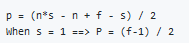
Same convolutions is a convolution with a pad so that output size is the same as the input size. Its given by the equation:
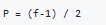
In computer vision f is usually odd. Some of the reasons is that its have a center value.
Strided convolution
Strided convolution is another piece that are used in CNNs
We will call stride s
When we are making the convolution operation we used s to tell us the number of pixels we will jump when we are convolving filter/kernel. The last examples we described s was 1
Now the general rule are:
if a matrix n*n is convolved with f*f filter/kernel and padding p and stride s it give us (n+2p-f)/s+1, (n+2p-f)/s+1 matrix
In case (n+2p-f)/s+1 is fraction we can take floor of this value.
In math textbooks the conv operation is filpping the filter before using it. What we were doing is called cross-correlation operation but the state of art of deep learning is using this as conv operation.
Same convolutions is a convolution with a pad so that output size is the same as the input size. Its given by the equation:
Convolution over volumes
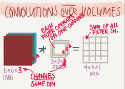
We see how convolution works with 2D images, now lets see if we want to convolve 3D iamges(RGB image)
We will convolve an image of height,width,# of channels with a filter of a height, width,same # of cahnnels. Hint hat the image number channels and the filter number of channels are the same.
We can call this as stacked filters for each channel!
Example
input image: 6*6*3
Filter:3*3*3
Result image: 4*4*1
In the last result p=0,s=1
Hint the output here is only 2D
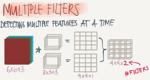
We can use multiple filters to detect multiple features or edges. Example
Input image: 6*6*3
10 Filters: 3*3*3
Result image: 4*4*10
In the last result p=0,s=1
One Layer of a Convolutional Network
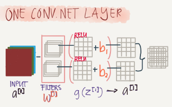
First we convolve some filters to a given input and then add a bias to each filter output and then get RELU of the result. Example:
Input iamge: 6*6*3 # a0
10 Filters: 3*3*3 #w1
Result image: 4*4*10 #w1a0
Add b(bias) with 10*1 will get us: 4*4*10 image #w1a0+b
Apply RELU will get us: 4*4*10 image #A1=RELU(w1a0+b)
In the last result p=0,s=1
Hint number of parameters here are; (3*3*3*10)+10=280
The last example forms a layer in the CNN
Hint that no matter how the size of the input, the number of the parameters for the same filter will still the same. That makes it less prune to overfitting
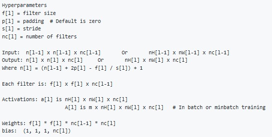
Here are some notation we will use. If layer l is a conv layer:
A simple convolution network example
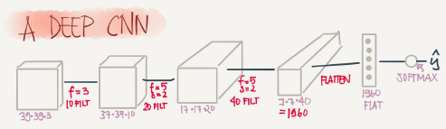
Lets build a big example.
Input Image are: a0=39*39*3
n0=39 and nc0=3
First layer(Conv layer):
f1=3,s1=1,and p1=0
number of filters=10
Then output are a1=37*37*10
n1=37 and nc1-10
second layer(Conv layer):
f2=5,s2=2,p2=0
number of filters=20
The output are a2=17*17*20
n2=17,nc2=20
Hint shrinking goes much faster because the stride is 2
Third layer(Conv layer):
f3=5,s3=2,p2=0
number of filters=40
The output are a3=7*7*40
n3=7,nc3=40
Forth layer(Fully connected softmax)
a3=7*7*40=1960 as a vector.
In the last example you seen that the image are getting smaller after each layer and that's the tread now.
Typesof layer in a convolutional network:
Convolution. #Conv
Pooling #Pool
Fully connected #FC
Pooling layers
Other than the conv layers,CNNs often uses pooling layers to reduce the size of the inputs, speed up computation, and to make some of the features it detects more robust.
Max pooling example:
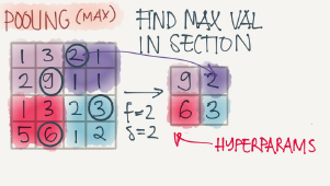
This example has f=2,s=2 and p=0 hyperparameters
The max pooling is saying, if the feature is detected anywhere in this filter then keep a high number. But the main reason why people are using pooling because its works well in practice and reduce computations.
Max pooling has no parameters to leran
Example of Max pooling on 3D input:
Input: 4*4*10
Max pooling size=2 and stride=2
output 2*2*10
Average pooling is taking the averages of the values instead of taking the max values
Max pooling is used more often than average pooling in practice.
If stride of pooling equals the size, it will then apply the effect of shrinking.
Hyperparameters summary
f: filter size
s: stride
Padding are rarely uses here
Max or average pooling
Convolutional neural network example
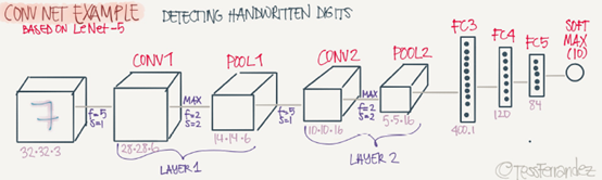
Now we will deal with a full CNN example. This example is something like the LeNet-5 that was invented by Yann Lecun
Input image are: a2=32*32*3
n0=32 and nc0=3
First layer(Conv layer): #Conv1
f1=5,s1=1,and p1=0
number of filters=6
Then output are a1=28*28*6
n1=28,and nc1=6
Then apply(Max pooling): #Pool1
f1p=2 and s1p=2
The output are a1=14*14*16
Second layer(Conv layer):#Conv2
f2=5,s2=1,p2=0
number of filters=16
The output are a2=10*10*16
n2=10,nc2=16
Then apply(Max pooling):#pool2
f1p=2,and s1p=2
The output are a2=5*5*16
Third layer(Fully connected) #FC3
Number of neurous are 120
The output a3=120*1, 400 came from 5*5*16
Forth layer(Full connected) #FC4
Number of neurons are 84
The output a4=84*1
Fifth layer(Softmax)
Number of neurons is 10 if we need to identify for example the 10 digits
Hint a Conv1 and Pool1 is treated as one layer
Some statistics about the last example:
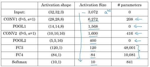
Hyperparameters are a lot. For choosing the value of each you should follow the guideline that we will discuss later or check the literature and takes some ideas and numbers from it.
Usually the input size decrease over layers while the number of filters incerease
A CNN usually consists of one or more convolution(Not just one as the shown examples) folowed by a pooling.
Fully connected layers has the most parameters in the network
To consider using these bolocks together you should look at other working examples firsts to get some intuitions
Why convollutions?
Two main advantages of Convs are:
Parameter sharing.
A feature detector(such as a vertical edge detector) that's useful in one part of the
image is probably useful in another part of the image
sparsity of connection.
In each layer, each output value depends only on a small number of inputs which
makes it translation
Putting it all together
Deep convolutional models: case studies
Learn about the practical tricks and methods used in deep CNNs straight from the research paper.
Why look at case studies?
We learned about Conv layer, pooling layer, and fully connected layers. It turns out that computer vision researchers spent the past few years on how to put these layers together.
To get some intuitions you have to see the examples that has been made.
Some neural networks architecture that works well in some tasks can also work well in other tasks.
Here are some classical CNN networks:
LeNet-5
AlexNet
VGG
The best CNN architecture that won the last ImageNet competition is called ResNet and it has 152 layers!
There are also an architecture called Inception that was made by Google that are very useful and apply to your tasks.
Reading and trying the mentioned models can boost you and give you a lot of ideas to solve your task.
Classic networks
In this section we will talk about classic networks which are LeNet-5,AlexNet, and VGG
LeNet-5
The goal for this model was to identify handwritten digits in a 32*32*1 gray image. Here are the drawing of it:
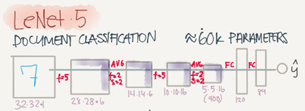
This model was published in 1998. The last layer wasn't using softmax back then
It has 60K parameters.
The dimensions of the image decreases as the number of channel s increases.
ConvèPoolèConvèPoolèFCèFCèsoftmax this type of arrangement is quite common.
The activation function used in the paper was Sigmoid and Tanh. Modern implementation uses RELU in most of the cases.
[LeCun et al., 1998. Gradient-based learning applied to document recognition]
AlexNet
Named after Alex Krizhevsky who was the first author of this paper. The other authors includes Jeoffery Hinton.
The goal for the model was the ImageNet challenge which classifies images into 1000 classes. Here are the drawing of the model:
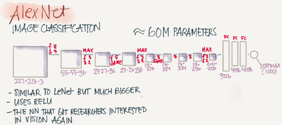
Summary:
ConvèMax-poolèConvèMax-poolèConvèConvèConvèMax-poolèFlattenèFCèFCèSoftmax
Similar to LeNet-5 but bigger.
Has 60 Million parameter compared to 60K parameter of LeNet-5
It used the RELU activation function.
The original paper contains Multiple GPUs and Local Response normalization(RN)
Multiple GPUs was used because the GPUs was so fast back then.
Researchers proved that Local Response normalization doesn't help much so far now
don't bother yoursef for understanding or implementing it.
This paper convinced the computer vision researchers that deep learning is so important.
VGG-16
A modification for AlexNet.
Instead of having a lot of hyperparameters lets have some simpler network.
Focus on having only these blocks:
CONV=3*3 filter, s=1, same
MAX-POOL=2*2,s=2
Here are the architecture:
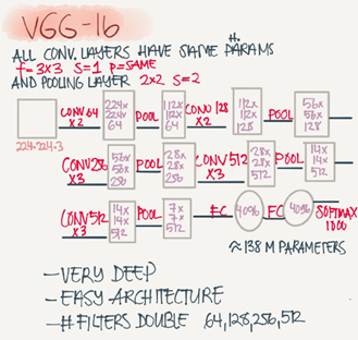
This network is large even by modern standards. It has around 138 million parameters.
Most of the paramters are in the fully connected layers.
It has a total memory of 96MB per image for only forward propagation!
Most memory are in the earlier layers.
Number of filters increases from 64 to 128 to 256 to 512, 512 was made twich.
Pooling was the only one who is responsible for shrinking the dimensions.
There are another version called VGG-19 which is bigger version. But most people used the VGG-16 instead of the VGG-19 because it does the same.
VGG paper is attractive it tries to make some rules regarding using CNNs
Special Netwroks
Residual Networks(ResNets)
Very, very deep NNs are difficult to train because of vanishing and exploding gradients problems.
In this section we will learn about skip connection which makes you take the activation from one layer and suddenly feed it to another layer even much deeper in NN which allows you to train large NNs even with layers greater than 100.
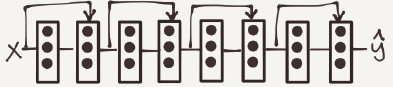
Residual block
ResNets are built out of some Residual blocks.
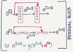
They add a shorcut/skip connection before the second activation.
The authors of this block find that you can train a deeper NNs using stacking this block.
Residual Network
Are a NN that consists of some Residual blocks.
These networks can go deeper without hurting the performance. In the normal NN –Plain networks- the theory tell us that if we go deeperwe will get a better solution to our problem. but because of the vanishing and exploding gradients problems the performance of the network suffers as it goes deeper. Thanks to Residual Network we can go deeper as we want now.
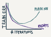
On the left is the normal NN and on the right are the ResNet. As you can see the performance of RestNet increases as the nwtwork goes deeper.
In some cases going deeper won't effect the performance and that depends on the problem on your hand.
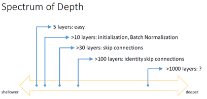
Some people are trying to train 1000 layer now which isn't used in practice
Why ResNets work
Lets see some example that illustrates why resNet work.
We have a big NN as the following:
XàBig NNàa[l]
Lets add two layers to this network as a residual block:
XàBig NNàa[l]àLayer1àLayer2àa[l+2]
And a[l] has a direct connection to a[a+2]
Suppose we are using RELU activations:
Then:
a[l+2]=g(z[l+2]+a[l])=g(w[l+2]a[l+1]+b[l+2]+a[l])
Then if we are using L2 regularization for example, w[l+2] will be zero. Lets say that b[l+2] will be zero too.
Then a[l+2]=g(a[l])=a[l] with no negative values.
This show that identity function is easy for a residual block to learn. And that why if can train deeper NNs.
Also that the two layers we added doesn't hurt the performance of big NN we made.
Hint: dimensions of z[l+2] and a[l] have to be the same in resNets. In case they have different dimension what we put a matrix parameters(Which can be learned or fixed)
a[l+2]=g(z[l+2]+ws*a[l]) #The added Ws should make the dimentions equal
ws also can be a zero padding
Using a skip-connection helps the gradient to backpropagate and thus heps you train deeper networks
Lets take a look at ResNet on images.
Here are the architecture of ResNet-34:
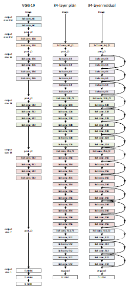
All the 3*3 Conv are same Convs
Keep it simple in design of the network
spatial size/2è #filters*2
No FC layers,No dropout is used
Two main types of blocks are used in a ResNet, depending mainly on whether the input/output dimensions are same of different. You are going to implement both of them.
The dotted lines is the case when the dimensions are different. To solve then they down sample the input by 2 and then pad zeros to match the two dimensions. There's another trick which is called bottleneck which we will explore later.
Useful concept(Spectrum of Depth)
Residual blocks types:
Identity block:
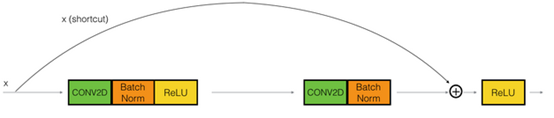
Hint the conv is followed by a batch norm BN before RELU. Dimensions here are the same.
This skip is over 2 layers. The skip connection can jump n connection where n>2
The convolutional block:
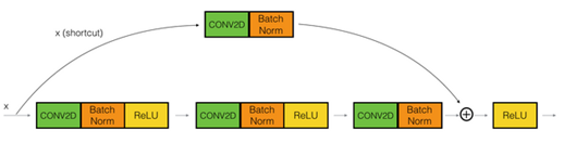
The conv can be bottleneck 1*1 conv
Network in Network and 1*1 convolutions
A 1*1 convolution- we also call it Network in Network- is so useful in many CNN models.
What does a 1*1 convolution do? Isn't it just multiplying by a number?
Let's first consider an example:
Input: 6*6*1
Conv:1*1*1 one filter. # The 1*1 Conv
Output: 6*6*1
Another example:
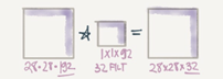
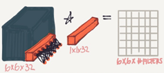
Input:6*6*32
Conv:1*1*32 5 filters. # The 1*1 Conv
Output: 6*6*5
It has been used in a lot of modern CNN implementations likes ResNet and Inception models.
A 1*1 convolution is sueful when:
we want to shrink the number of channels. We also call this feature transformation.
In the second discussed example above we have shrieked the input from 32 to 5
We will later see that by shrinking it can save a lot of computations
If we have specified the number of 1*1 Conv filters to be the same as the input number
of channels then the output will contain the same number of channels. Then 1*1 Conv will act like a non linearity and will learn non linearity operator.
Replace fully connected layers with 1*1 convolutions as Yann LeCun believes they are the same.
In Convolutional Nets, there is no such thing as "fully-connected layers", There are only
convolution layers with 1*1 convolution kernel and a full connection table.
Inception network motivation
When you design a CNN you have to decide all the layers yourself. Will you pick a 3*3 Conv or 5*5 Conv or maybe a max pooling layer. You have so many choices.
What inception tells us is, Why not use all of them at once?
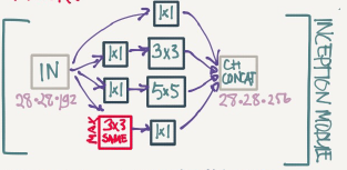
Inception module, naïve version:
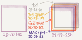
Hint that max-pool are same here.
Input to the inception module are 28*28*192 and the output are 28*28*256
We have done all the Convs and pools we might want and will let the NN learn and decide which it want to use most.
The problem of computational cost in Inception model:
If we have just focused on a 5*5 Conv that we have done in the last example.
There are 32 same filters of 5*5, and the input are 28*28*192
output should be 28*28*32
The total number of multiples needed here are:
Number of output*Filter size*Filter size*Input dimensions
Which equals: 28*28*32*5*5*192=120Mil
120Mil multiply operation still a problem in the modern day computers.
Using a 1*1 convolution we can reduce 120mil to just 12 mil. Lets see how.
Using 1*1 convolution to reduce computational cost:
The new architecture are:
X0 shape is (28,28,192)
We then apply 16(1*1 Convolution)
That produces X1 of shape (28,28,16)
Hint, we have reduced the dimensions here.
Then apply 32(5*5 Convolution)
That produces X2 of shape(28,28,32)
Now lets calculate the number of multiplications:
For the first Conv: 28*28*16*1*1*192=2.5Mil
For the second Conv: 28*28*32*5*5*16=10Mil
So the total number are 12.5Mil approx. Which is so good compared to 120Mil
A 1*1 Conv here is called Bottlenect BN
It turns out that the 1*1 Conv won't hurt the performance.
Inception module,dimensions reduction version:
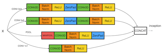
Example of inception model in Keras:
Inception network(GoodNet)
The inception network consist of concatenated blocks of the Inception module.
The name inception was taken from a name image which was taken from Inception movie
There are the full model:
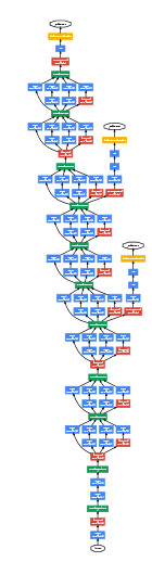
Some times a Max-pool block is used before the inception module to reduce the dimensions of the inputs.
There are a 3 Sofmax branches at different positions to push the network toward its goal. and helps to ensure that the intermediate features are good enough to the network to learn and it turns out that softmax0 and softmax1 gives regularization effect.
Since the development of the inception module, the authors and the others have built another versions of this network. Like inception v2,v3 and v4. Also there are a network that has used the inception module and the ResNet together.