论文《Piexel Recurrent Nerual Network》总结

论文：《Pixel Recurrent Nerual Network》

时间：2016

作者：Aaron van den Oord, Nal Kalchbrenner, Koray Kavukcuoglu

期刊：CCF A类会议 ICML

谷歌学术引用量：326

意义：将RNN和CNN用于像素的生成

由于这篇论文在阅读的时候有一些前置知识不是很懂，因此根据这篇论文的引用，以及引用论文的引用论文大概略读了以下论文

[1]Theis, Lucas, and Matthias Bethge. "Generative image modeling using spatial LSTMs." Advances in Neural Information Processing Systems. 2015.

[2]Williams, R. J., and D. Zipser. "Gradient-based learning algorithm for recurrent connectionist networks." Northern Univ., College Comp. Sci. Tech. Rep., NU-CCs-90-9 (1990).

[3]Graves, Alex, and Jürgen Schmidhuber. "Offline handwriting recognition with multidimensional recurrent neural networks." Advances in neural information processing systems. 2009.

[4]Graves, Alex, S. Fernández, and J. Schmidhuber. "Multi-dimensional Recurrent Neural Networks." International Conference on Artificial Neural Networks Springer, Berlin, Heidelberg, 2007:549-558.

[5]Theis, Lucas, R. Hosseini, and M. Bethge."Mixtures of Conditional Gaussian Scale Mixtures Applied Multiscale Image Representations." Plos One 7.7(2011):e39857.

Mulit-Dimensional Recurrent Neural Networks

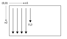
在理解《Pixel Recurrent Nerual Network》之前需要明白论文《Multi-dimensional Recurrent Neural Networks》的几个概念。简单的说一下论文《Multi-dimensional Recurrent Neural Networks》将LSTM的维度扩展成多个维度。在前向传播的时候，在数据序列上的每一个点，在神经网络隐藏层上收到一个外在的输入和它自己在前一步所有维度的激活元（activations）。

具体的过程如Figure 1：2D RNN Forward pass 所示。

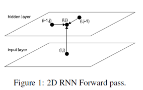
很显然，数据必须在收到之前的激活元（activations）时，这些激活元必须已经生成了。

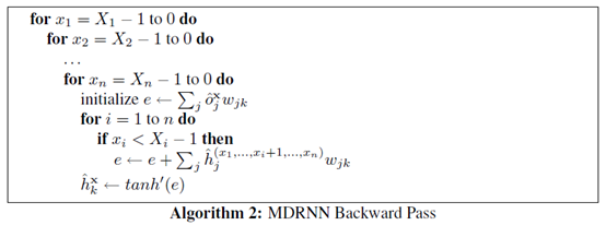
在反向传播的每一个tiemstep,隐藏层收到的数据来自两个方面，一个是error derivatives和另一个是'future' derivatives。下图展示了两个维度的反向传播过程。

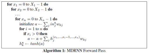
MDRNN（Multi-Dimensional Recurrent Nerual Networks）的前向和反向传播算法过程如下:

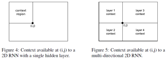
Multi-directional MDRNNs

在很早的时候就提出了BRNN（bidirectional recurrent neural networks）双向循环神经网络。可以将双向的循环神经网络的思想扩展到n维，使用分离的隐藏层

MCGSM(Mixtures of conditional Gaussian scale mixtures)

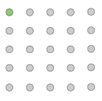
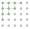
按照常规的思路我们生成下一个像素的时候，会依赖于之前的所有像素。

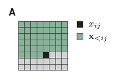
黑色是我们要生成的像素，绿色是之前的所有像素。

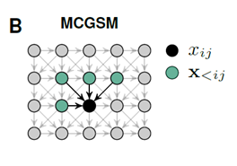
论文《Mixtures of conditional Gaussian scale mixtures applied to multiscale iamge representations》提出了MCGSM用于图像的生成，该思想简单的说，就是生成该像素只依赖于他周边之前的像素点

Spatial LSTMs

论文《Generative Image Modeling Using Spatial LSTMs》提出了Spatial LSTMs用于图像的生成。简单的说Spatial LSTMs 是一个两个维度的LSTM。

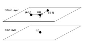
Spatial LSTMs用于像素的生成过程如下

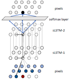
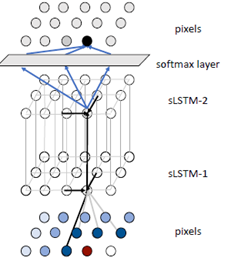
底层是输入的数据采用MCGSM获得数据传向中间层Spatial LSTM，中间层的Spatial LSTM通过MDRNN的前向传播算法计算出当前点的值传给第二层Spatial LSTM,最后一层连接softmax layer 会输出255个值。在softmax layer中采用采样算法获取当前点的生成。

Piexel Recurrent Nerual Network

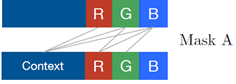
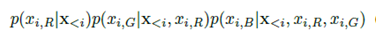
有了前面的前置知识之后就可以阅读论《Piexel Recurrent Nerual Network》。因为数据生成是通过之前的生成的点来进行生成的。因此论文提出了两种Mask(Mack A, Mask B)用于屏蔽未来的数据对当前数据的影响。

MaskA：只使用之前的数据，而不使用自己的R,G,B的值进行生成。

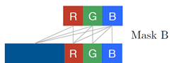
MaskB: 使用之前的数据，并且使用自己的R,G,B的值进行生成。

MaskA的数据表示形式如下

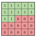
如果是MaskB的话，最中心的值为1

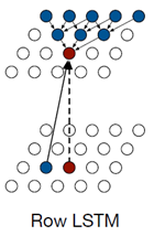
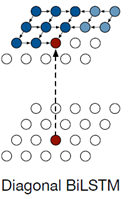
论文还提出了自己的LSTM结构Row LSTM 以及 Diagonal BiLSTM

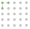
Row LSTM: Row LSTM每个点的生成依赖于前面的三个点。

Diagonal BiLSTM:首先Diagonal BiLSTM是一个双向链表，其次每次扩展的时候都会沿着这个方向进行

论文还提出了PixelCNN

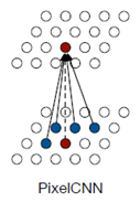
PixelCNN和普通的CNN的区别是在进行卷积操作的时候，会先和前面提到的mask进行相乘，取消掉将来点的影响。

有了这些知识就可以生成图片了，通过Diagonal BiLSTM图片直观的生成顺序如下

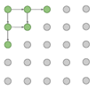
沿着左上角一直往右下角生成

网络的整体结构论文给出了如下的结构

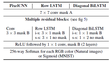
和前面提到的Spatial LSTMs用于生成图片的结构有点像，只是LSTM使用的是论文自己设计出来的Row LSTM或者Diagonal BiLSTM。在LSTM层的前面和后面多了几层PixelCNN层。

PiexelCNN的实现

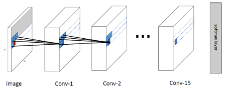
由于PiexelRNN是多层的LSTM结构计算量过于庞大，没有高性能的计算机无法实现。下面用PiexelCNN实现图像的生成。

该模型的整体结构如下

下面给出了PiexelCNN的核心代码

构造PixelCNN卷积层的代码

def conv2d(
inputs,
num_outputs,
kernel_shape, # [kernel_height, kernel_width]
mask_type, # None, "A" or "B",mask的类别
strides=[1, 1], # [column_wise_stride, row_wise_stride]
padding="SAME",
activation_fn=None,
weights_initializer=WEIGHT_INITIALIZER,
weights_regularizer=None,
biases_initializer=tf.zeros_initializer,
biases_regularizer=None,
scope="conv2d"):
with tf.variable_scope(scope):
mask_type = mask_type.lower()
batch_size, height, width, channel = inputs.get_shape().as_list()

kernel_h, kernel_w = kernel_shape
stride_h, stride_w = strides

assert kernel_h % 2 == 1 and kernel_w % 2 == 1,
"kernel height and width should be odd number"

center_h = kernel_h // 2
center_w = kernel_w // 2

weights_shape = [kernel_h, kernel_w, channel, num_outputs]
weights = tf.get_variable("weights", weights_shape,
tf.float32, weights_initializer, weights_regularizer)

if mask_type is not None:
mask = np.ones(
(kernel_h, kernel_w, channel, num_outputs), dtype=np.float32)

mask[center_h, center_w+1: ,: ,:] = 0.
mask[center_h+1:, :, :, :] = 0.

if mask_type == 'a':
mask[center_h,center_w,:,:] = 0.

weights *= tf.constant(mask, dtype=tf.float32)
tf.add_to_collection('conv2d_weights_%s' % mask_type, weights)

outputs = tf.nn.conv2d(inputs,
weights, [1, stride_h, stride_w, 1], padding=padding, name='outputs')
tf.add_to_collection('conv2d_outputs', outputs)

if biases_initializer != None:
biases = tf.get_variable("biases", [num_outputs,],
tf.float32, biases_initializer, biases_regularizer)
outputs = tf.nn.bias_add(outputs, biases, name='outputs_plus_b')

if activation_fn:
outputs = activation_fn(outputs, name='outputs_with_fn')
return outputs

PixelCNN网络的整体结构构造

#构造输入层PixelCNN

self.l[scope] = conv2d(self.l['normalized_inputs'], conf.hidden_dims, [7, 7], "A", scope=scope)

#构造中间几层的PixelCNN

l_hid = self.l[scope]
for idx in range(conf.recurrent_length):
    scope = 'CONV%d' % idx

													self.l[scope] = l_hid = conv2d(l_hid, 3, [3, 3], "B", scope=scope)
#构造输出层的PixelCNN

for idx in range(conf.out_recurrent_length):
  scope = 'CONV_OUT%d' % idx

										self.l[scope] = l_hid = tf.nn.relu(conv2d(l_hid, conf.out_hidden_dims, [1, 1], "B", scope=scope))

#构造输出层的softmax layer

self.l['conv2d_out_logits'] = conv2d(l_hid, 1, [1, 1], "B", scope='conv2d_out_logits')
self.l['output'] = tf.nn.sigmoid(self.l['conv2d_out_logits'])

#损失函数

self.loss = tf.reduce_mean(tf.nn.sigmoid_cross_entropy_with_logits(

						logits=self.l['conv2d_out_logits'], labels=self.l['normalized_inputs'], name='loss'))