Convolutions in TensorFlow

Convolutions in TensorFlow

Convolutions without training

You might already be familiar with the term "convolution" from a mathematical or physical context. In the mathematical context, "convolution" is defined, by Oxford dictionary, as followed:

a function derived from two given functions by integration that expresses

how the shape of one is modified by the other.

Gif source: Wikipedia

And that's pretty much what convolution means in the machine learning context. Convolution is how the original input is modified by the kernel (or filter/feature map). To better understand convolutions, Chris Olah has a detailed blog post with illustrations.

Source gif: http://deeplearning.stanford.edu/.

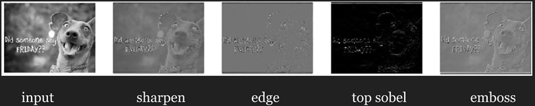
We can, in fact, do convolution without training. For example, we can choose a kernel and see how that kernel transforms our image. For example, a common kernel used for blurring an image is a square matrix of dimension 3 x 3 with the values as below. When you slide the kernel across an image and multiply the kernel with different parts of image directly under the kernel, the result is a weighted sum of neighboring pixels, which leads to the blurring effect.

To do convolution in TensorFlow, there are several built-in layers we can use. You can do either one-dimensional convolution (input is 2 dimension), two-dimensional convolution (input is 3 dimension), or three-dimensional convolution (input is 4 dimension). For most of our purposes, we will be concerning ourselves with 2D convolution. For illustration of convolution with inputs of different dimensions, please see runhani's StackOverflow answer.

tf.nn.conv2d(

input,

filter,

strides,

padding,

use_cudnn_on_gpu=True,

data_format='NHWC',

dilations=[1, 1, 1, 1],

name=None

)

Input: Batch size (N) x Height (H) x Width (W) x Channels (C)

Filter: Height x Width x Input Channels x Output Channels

(e.g. [5, 5, 3, 64])

Strides: 4 element 1-D tensor, strides in each direction

(often [1, 1, 1, 1] or [1, 2, 2, 1])

Padding: 'SAME' or 'VALID'

Dilations: The dilation factor. If set to k > 1, there will be k-1 skipped cells between each filter element on that dimension.

Data_format: default to NHWC

For strides, you don't want to use any number other than 1 in the first and the fourth dimension since you don't want to skip any sample in a batch, or any channel in an image. The same for dilations.

There are several other built-in convolutional operations. Please refer to the official documentation for more information.

conv2d: Filters that mix channels together.

depthwise_conv2d: Filters that operate on each channel independently.

separable_conv2d: A depthwise spatial filter followed by a pointwise filter.

As a fun exercise, you can see the values of several other popular kernels in the file kernels.py on the class GitHub repository, and see how to use them in 07_basic_kernels.py.

In this exercises, we hard-coded the values of our kernels. When training a convnet, we don't know in advance the optimal values for our kernels and therefore have to learn them. We'll go through the process of learning the kernels through a simple convnet with our old friend MNIST.

Convnet on MNIST

We've done logistic regression with a single fully connected layer on MNIST and the result is abysmal. Let's see if a convnet with locally connected layers would do better.

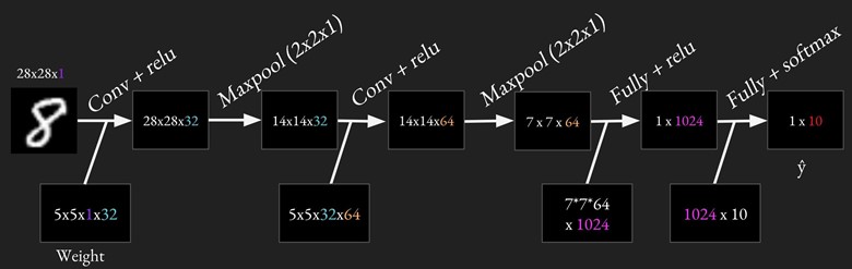
For MNIST, we will be using two convolutional layers, each followed by a relu and a maxpool layers, and two fully connected layers. Strides for all convolutional layers are [1, 1, 1, 1].

Because will do the same things multiple times (e.g. conv + relu twice, max pooling twice, fully connected twice), it's a good idea to have reusable code. It's also important to use variable scope so we can have variables with the same names for different layers. A variable name 'weights' in variable scope 'conv1' will become 'conv1/weights'. The common practice is to create a variable scope for each layer, so that if you have variable 'weights' in both convolution layer 1 and convolution layer 2, there won't be any name clash. If you're still unsure about variable scope, please see Variable sharing in Lecture note 05.

Convolutional layer

We will be using tf.nn.conv2d for the convolutional layer. A common practice is to group convolutional layer and non-linearity together, which we will do in this case. We will create a method conv_relu that can be used for both convolutional layers.

def conv_relu(inputs, filters, k_size, stride, padding, scope_name):

with tf.variable_scope(scope_name, reuse=tf.AUTO_REUSE) as scope:

in_channels = inputs.shape[-1]

kernel = tf.get_variable('kernel', [k_size, k_size, in_channels, filters],

initializer=tf.truncated_normal_initializer())

biases = tf.get_variable('biases', [filters],

initializer=tf.random_normal_initializer())

conv = tf.nn.conv2d(inputs, kernel, strides=[1, stride, stride, 1], padding=padding)

return tf.nn.relu(conv + biases, name=scope.name)

We don't have to manually calculate the dimension (the spatial size) of the output, but it's a good idea to do so to keep a mental account of how our inputs are being transformed at each step. We can compute the spatial size on each dimension (width/depth) as a function of:

• the input volume size (W)
• the receptive field size of filter (F)
• the stride with which they are applied (S)
• the amount of zero padding used (P) on the border.

The formula is as followed:

 

For example for a 7x7 input and a 3x3 filter with stride 1 and pad 0 we would get a 5x5 output. With stride 2 we would get a 3x3 output. In our case, for the first convolutional layer, we have:

• input of size 28x28
• filter size 5x5
• stride 1x1
• padding (done automatically for us) 2

So the spatial size of the output would be:

 

A nice illustration to see how striding affect the dimensionality of the outside. For full analysis, see CS231N's lecture note.

 

Pooling

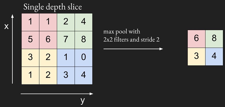
Pooling is a downsampling technique to reduce the dimensionality of the feature map extracted from the convolutional layer in order to reduce the processing time. Pooling layers replace a subregion of data with (hopefully) its most representative feature. The most popular pooling algorithm, max pooling, replaces a subregion of data with its maximal value. Another algorithm is average pooling, when we averages all the values in one subregion to have one single value.

We will be using tf.nn.max_pool for the max pooling layer. We will create a method maxpool that can be used for both pooling layers.

def maxpool(inputs, ksize, stride, padding='VALID', scope_name='pool'):

with tf.variable_scope(scope_name, reuse=tf.AUTO_REUSE) as scope:

pool = tf.nn.max_pool(inputs,

ksize=[1, ksize, ksize, 1],

strides=[1, stride, stride, 1],

padding=padding)

return pool

We can compute the spatial size on each dimension (width/depth) of the output of pooling layer a function of:

• the input volume size (W)
• the pooling size (K)
• the stride with which they are applied (S)
• the amount of zero padding used (P) on the border.

The formula is as followed:

 

In our case, for the first max pooling layer, we have:

• input of size 28x28
• pooling size 2 x 2
• stride 2 x 2
• padding (done automatically for us) 0

So the spatial size of the output would be:

 

Fully connected

We should be pretty familiar with the fully connected layer by now, as we have been using it for all of our models. Fully connected, or dense, layer is called so because every node in the layer is connected to every node in the preceding layer. Convolutional layers are only locally connected.

def fully_connected(inputs, out_dim, scope_name='fc'):

with tf.variable_scope(scope_name, reuse=tf.AUTO_REUSE) as scope:

in_dim = inputs.shape[-1]

w = tf.get_variable('weights', [in_dim, out_dim],

initializer=tf.truncated_normal_initializer())

b = tf.get_variable('biases', [out_dim],

initializer=tf.constant_initializer(0.0))

out = tf.matmul(inputs, w) + b

return out

Putting it together

With those building blocks (layers), we can easily construct our model.

def inference(self):

conv1 = conv_relu(inputs=self.img,

filters=32,

k_size=5,

stride=1,

padding='SAME',

scope_name='conv1')

pool1 = maxpool(conv1, 2, 2, 'VALID', 'pool1')

conv2 = conv_relu(inputs=pool1,

filters=64,

k_size=5,

stride=1,

padding='SAME',

scope_name='conv2')

pool2 = maxpool(conv2, 2, 2, 'VALID', 'pool2')

feature_dim = pool2.shape[1] * pool2.shape[2] * pool2.shape[3]

pool2 = tf.reshape(pool2, [-1, feature_dim])

fc = tf.nn.relu(fully_connected(pool2, 1024, 'fc'))

dropout = tf.layers.dropout(fc, self.keep_prob, training=self.training, name='dropout')

self.logits = fully_connected(dropout, self.n_classes, 'logits')

During training, we alternate between training an epoch and evaluating the accuracy on the test set. We will track both the training loss and test accuracy on Tensorboard.

def eval(self):

'''

Count the number of right predictions in a batch

'''

with tf.name_scope('predict'):

preds = tf.nn.softmax(self.logits)

correct_preds = tf.equal(tf.argmax(preds, 1), tf.argmax(self.label, 1))

self.accuracy = tf.reduce_sum(tf.cast(correct_preds, tf.float32))

See the full code on the class's GitHub under the name 07_convnet_mnist.py

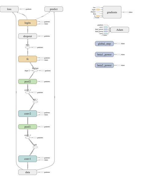
Don't you love it when your graph comes together neatly like this!

The number of right predictions for each test batch steadily increases as the train loss decreases.

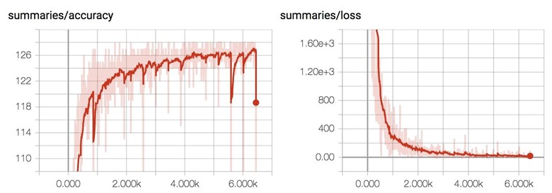
Below is the training result for MNIST with our convolutional neural network. We got much better accuracy, but it also takes a lot longer to train, approximately 250 seconds an epoch! It's expected since the model has to do a lot more computation per step now.

Epochs	Accuracy
1	0.9131
2	0.9363
3	0.9478
5	0.9573
10	0.971
25	0.9818

tf.layers

I have a confession to make: we've been learning how to do it the hard way. We actually don't have to write the conv_relu method, pooling, or fully_connected. TensorFlow has a module called tf.layers that provides many off-the-shelf layers. Higher level libraries like Keras, Sonnet also provide ready-made models that you can call with a few lines of code.

For example, to create a convolutional layer with relu non-linearity on the input image, we can call:

conv1 = tf.layers.conv2d(inputs=self.img,

filters=32,

kernel_size=[5, 5],

padding='SAME',

activation=tf.nn.relu,

name='conv1')

tf.layers.conv2d let you choose the activation function to use.

For max pooling and fully connected, we can call:

pool1 = tf.layers.max_pooling2d(inputs=conv1,

pool_size=[2, 2],

strides=2,

name='pool1')

fc = tf.layers.dense(pool2, 1024, activation=tf.nn.relu, name='fc')

It's pretty straightforward to use tf.layers. There's only one tiny thing to note. With tf.layers.dropout, you need to have another variable to indicate whether it's in the training mode or in the evaluation mode. We want to drop out neurons during training, but we want to use all of them during evaluating!

dropout = tf.layers.dropout(fc,

self.keep_prob,

training=self.training,

name='dropout')

You get the idea! For the full list of layers that tf.layers provides, feel free to head to the official documentation.