Advice for Applying Machine Learning
Applying machine learning in practice is not always straightforward. In this module, we share best practices for applying machine learning in practice, and discuss the best ways to evaluate performance of the learned models.
7 videos, 7 readings
Video: Deciding What to Try Next
By now you have seen a lot of different learning algorithms.
0:03
And if you've been following along these videos you should consider yourself an expert on many state-of-the-art machine learning techniques. But even among people that know a certain learning algorithm. There's often a huge difference between someone that really knows how to powerfully and effectively apply that algorithm, versus someone that's less familiar with some of the material that I'm about to teach and who doesn't really understand how to apply these algorithms and can end up wasting a lot of their time trying things out that don't really make sense.
0:34
What I would like to do is make sure that if you are developing machine learning systems, that you know how to choose one of the most promising avenues to spend your time pursuing. And on this and the next few videos I'm going to give a number of practical suggestions, advice, guidelines on how to do that. And concretely what we'd focus on is the problem of, suppose you are developing a machine learning system or trying to improve the performance of a machine learning system, how do you go about deciding what are the proxy avenues to try
1:07
next?
1:09
To explain this, let's continue using our example of learning to predict housing prices. And let's say you've implement and regularize linear regression. Thus minimizing that cost function j. Now suppose that after you take your learn parameters, if you test your hypothesis on the new set of houses, suppose you find that this is making huge errors in this prediction of the housing prices.
1:33
The question is what should you then try mixing in order to improve the learning algorithm?
1:39
There are many things that one can think of that could improve the performance of the learning algorithm.
1:44
One thing they could try, is to get more training examples. And concretely, you can imagine, maybe, you know, setting up phone surveys, going door to door, to try to get more data on how much different houses sell for.
1:57
And the sad thing is I've seen a lot of people spend a lot of time collecting more training examples, thinking oh, if we have twice as much or ten times as much training data, that is certainly going to help, right? But sometimes getting more training data doesn't actually help and in the next few videos we will see why, and we will see how you can avoid spending a lot of time collecting more training data in settings where it is just not going to help.
2:22
Other things you might try are to well maybe try a smaller set of features. So if you have some set of features such as x1, x2, x3 and so on, maybe a large number of features. Maybe you want to spend time carefully selecting some small subset of them to prevent overfitting.
2:38
Or maybe you need to get additional features. Maybe the current set of features aren't informative enough and you want to collect more data in the sense of getting more features.
2:48
And once again this is the sort of project that can scale up the huge projects can you imagine getting phone surveys to find out more houses, or extra land surveys to find out more about the pieces of land and so on, so a huge project. And once again it would be nice to know in advance if this is going to help before we spend a lot of time doing something like this. We can also try adding polynomial features things like x2 square x2 square and product features x1, x2. We can still spend quite a lot of time thinking about that and we can also try other things like decreasing lambda, the regularization parameter or increasing lambda.
3:23
Given a menu of options like these, some of which can easily scale up to six month or longer projects.
3:31
Unfortunately, the most common method that people use to pick one of these is to go by gut feeling. In which what many people will do is sort of randomly pick one of these options and maybe say, "Oh, lets go and get more training data." And easily spend six months collecting more training data or maybe someone else would rather be saying, "Well, let's go collect a lot more features on these houses in our data set." And I have a lot of times, sadly seen people spend, you know, literally 6 months doing one of these avenues that they have sort of at random only to discover six months later that that really wasn't a promising avenue to pursue.
4:07
Fortunately, there is a pretty simple technique that can let you very quickly rule out half of the things on this list as being potentially promising things to pursue. And there is a very simple technique, that if you run, can easily rule out many of these options,
4:24
and potentially save you a lot of time pursuing something that's just is not going to work.
4:29
In the next two videos after this, I'm going to first talk about how to evaluate learning algorithms.
4:36
And in the next few videos after that, I'm going to talk about these techniques,
4:42
which are called the machine learning diagnostics.
4:46
And what a diagnostic is, is a test you can run, to get insight into what is or isn't working with an algorithm, and which will often give you insight as to what are promising things to try to improve a learning algorithm's
5:03
performance. We'll talk about specific diagnostics later in this video sequence. But I should mention in advance that diagnostics can take time to implement and can sometimes, you know, take quite a lot of time to implement and understand but doing so can be a very good use of your time when you are developing learning algorithms because they can often save you from spending many months pursuing an avenue that you could have found out much earlier just was not going to be fruitful.
5:32
So in the next few videos, I'm going to first talk about how evaluate your learning algorithms and after that I'm going to talk about some of these diagnostics which will hopefully let you much more effectively select more of the useful things to try mixing if your goal to improve the machine learning system.
Video: Evaluating a Hypothesis
In this video, I would like to talk about how to evaluate a hypothesis that has been learned by your algorithm. In later videos, we will build on this to talk about how to prevent in the problems of overfitting and underfitting as well. When we fit the parameters of our learning algorithm we think about choosing the parameters to minimize the training error. One might think that getting a really low value of training error might be a good thing, but we have already seen that just because a hypothesis has low training error, that doesn't mean it is necessarily a good hypothesis. And we've already seen the example of how a hypothesis can overfit. And therefore fail to generalize the new examples not in the training set. So how do you tell if the hypothesis might be overfitting. In this simple example we could plot the hypothesis h of x and just see what was going on. But in general for problems with more features than just one feature, for problems with a large number of features like these it becomes hard or may be impossible to plot what the hypothesis looks like and so we need some other way to evaluate our hypothesis. The standard way to evaluate a learned hypothesis is as follows. Suppose we have a data set like this. Here I have just shown 10 training examples, but of course usually we may have dozens or hundreds or maybe thousands of training examples. In order to make sure we can evaluate our hypothesis, what we are going to do is split the data we have into two portions. The first portion is going to be our usual training set
1:42
and the second portion is going to be our test set, and a pretty typical split of this all the data we have into a training set and test set might be around say a 70%, 30% split. Worth more today to grade the training set and relatively less to the test set. And so now, if we have some data set, we run a sine of say 70% of the data to be our training set where here "m" is as usual our number of training examples and the remainder of our data might then be assigned to become our test set. And here, I'm going to use the notation m subscript test to denote the number of test examples. And so in general, this subscript test is going to denote examples that come from a test set so that x1 subscript test, y1 subscript test is my first test example which I guess in this example might be this example over here. Finally, one last detail whereas here I've drawn this as though the first 70% goes to the training set and the last 30% to the test set. If there is any sort of ordinary to the data. That should be better to send a random 70% of your data to the training set and a random 30% of your data to the test set. So if your data were already randomly sorted, you could just take the first 70% and last 30% that if your data were not randomly ordered, it would be better to randomly shuffle or to randomly reorder the examples in your training set. Before you know sending the first 70% in the training set and the last 30% of the test set. Here then is a fairly typical procedure for how you would train and test the learning algorithm and the learning regression. First, you learn the parameters theta from the training set so you minimize the usual training error objective j of theta, where j of theta here was defined using that 70% of all the data you have. There is only the training data. And then you would compute the test error. And I am going to denote the test error as j subscript test. And so what you do is take your parameter theta that you have learned from the training set, and plug it in here and compute your test set error. Which I am going to write as follows. So this is basically the average squared error as measured on your test set. It's pretty much what you'd expect. So if we run every test example through your hypothesis with parameter theta and just measure the squared error that your hypothesis has on your m subscript test, test examples. And of course, this is the definition of the test set error if we are using linear regression and using the squared error metric. How about if we were doing a classification problem and say using logistic regression instead. In that case, the procedure for training and testing say logistic regression is pretty similar first we will do the parameters from the training data, that first 70% of the data. And it will compute the test error as follows. It's the same objective function as we always use but we just logistic regression, except that now is define using our m subscript test, test examples. While this definition of the test set error j subscript test is perfectly reasonable. Sometimes there is an alternative test sets metric that might be easier to interpret, and that's the misclassification error. It's also called the zero one misclassification error, with zero one denoting that you either get an example right or you get an example wrong. Here's what I mean. Let me define the error of a prediction. That is h of x. And given the label y as equal to one if my hypothesis outputs the value greater than equal to five and Y is equal to zero or if my hypothesis outputs a value of less than 0.5 and y is equal to one, right, so both of these cases basic respond to if your hypothesis mislabeled the example assuming your threshold at an 0.5. So either thought it was more likely to be 1, but it was actually 0, or your hypothesis stored was more likely to be 0, but the label was actually 1. And otherwise, we define this error function to be zero. If your hypothesis basically classified the example y correctly. We could then define the test error, using the misclassification error metric to be one of the m tests of sum from i equals one to m subscript test of the error of h of x(i) test comma y(i). And so that's just my way of writing out that this is exactly the fraction of the examples in my test set that my hypothesis has mislabeled. And so that's the definition of the test set error using the misclassification error of the 0 1 misclassification metric. So that's the standard technique for evaluating how good a learned hypothesis is. In the next video, we will adapt these ideas to helping us do things like choose what features like the degree polynomial to use with the learning algorithm or choose the regularization parameter for learning algorithm.
Reading: Evaluating a Hypothesis
Evaluating a Hypothesis
Once we have done some trouble shooting for errors in our predictions by:
- Getting more training examples
- Trying smaller sets of features
- Trying additional features
- Trying polynomial features
- Increasing or decreasing (lambda)
We can move on to evaluate our new hypothesis.
A hypothesis may have a low error for the training examples but still be inaccurate (because of overfitting). Thus, to evaluate a hypothesis, given a dataset of training examples, we can split up the data into two sets: a training set and a test set. Typically, the training set consists of 70 % of your data and the test set is the remaining 30 %.
The new procedure using these two sets is then:
- Learn (Theta) and minimize (J_{train}(Theta)) using the training set
- Compute the test set error (J_{test}(Theta))
The test set error
- For linear regression: (J_{test}(Theta) = dfrac{1}{2m_{test}} sum_{i=1}^{m_{test}}(h_Theta(x^{(i)}_{test}) - y^{(i)}_{test})^2)
- For classification ~ Misclassification error (aka 0/1 misclassification error):

This gives us a binary 0 or 1 error result based on a misclassification. The average test error for the test set is:
( ext{Test Error} = dfrac{1}{m_{test}} sum^{m_{test}}_{i=1} err(h_Theta(x^{(i)}_{test}), y^{(i)}_{test}))
This gives us the proportion of the test data that was misclassified.
Video: Model Selection and Train/Validation/Test Sets
Suppose you're left to decide what degree of polynomial to fit to a data set. So that what features to include that gives you a learning algorithm. Or suppose you'd like to choose the regularization parameter longer for learning algorithm. How do you do that? This account model selection process. Browsers, and in our discussion of how to do this, we'll talk about not just how to split your data into the train and test sets, but how to switch data into what we discover is called the train, validation, and test sets. We'll see in this video just what these things are, and how to use them to do model selection. We've already seen a lot of times the problem of overfitting, in which just because a learning algorithm fits a training set well, that doesn't mean it's a good hypothesis. More generally, this is why the training set's error is not a good predictor for how well the hypothesis will do on new example. Concretely, if you fit some set of parameters. Theta0, theta1, theta2, and so on, to your training set. Then the fact that your hypothesis does well on the training set. Well, this doesn't mean much in terms of predicting how well your hypothesis will generalize to new examples not seen in the training set. And a more general principle is that once your parameter is what fit to some set of data. Maybe the training set, maybe something else. Then the error of your hypothesis as measured on that same data set, such as the training error, that's unlikely to be a good estimate of your actual generalization error. That is how well the hypothesis will generalize to new examples. Now let's consider the model selection problem. Let's say you're trying to choose what degree polynomial to fit to data. So, should you choose a linear function, a quadratic function, a cubic function? All the way up to a 10th-order polynomial.
1:51
So it's as if there's one extra parameter in this algorithm, which I'm going to denote d, which is, what degree of polynomial. Do you want to pick. So it's as if, in addition to the theta parameters, it's as if there's one more parameter, d, that you're trying to determine using your data set. So, the first option is d equals one, if you fit a linear function. We can choose d equals two, d equals three, all the way up to d equals 10. So, we'd like to fit this extra sort of parameter which I'm denoting by d. And concretely let's say that you want to choose a model, that is choose a degree of polynomial, choose one of these 10 models. And fit that model and also get some estimate of how well your fitted hypothesis was generalize to new examples. Here's one thing you could do. What you could, first take your first model and minimize the training error. And this would give you some parameter vector theta. And you could then take your second model, the quadratic function, and fit that to your training set and this will give you some other. Parameter vector theta. In order to distinguish between these different parameter vectors, I'm going to use a superscript one superscript two there where theta superscript one just means the parameters I get by fitting this model to my training data. And theta superscript two just means the parameters I get by fitting this quadratic function to my training data and so on. By fitting a cubic model I get parenthesis three up to, well, say theta 10. And one thing we ccould do is that take these parameters and look at test error. So I can compute on my test set J test of one, J test of theta two, and so on.
3:47
J test of theta three, and so on.
3:53
So I'm going to take each of my hypotheses with the corresponding parameters and just measure the performance of on the test set. Now, one thing I could do then is, in order to select one of these models, I could then see which model has the lowest test set error. And let's just say for this example that I ended up choosing the fifth order polynomial. So, this seems reasonable so far. But now let's say I want to take my fifth hypothesis, this, this, fifth order model, and let's say I want to ask, how well does this model generalize?
4:27
One thing I could do is look at how well my fifth order polynomial hypothesis had done on my test set. But the problem is this will not be a fair estimate of how well my hypothesis generalizes. And the reason is what we've done is we've fit this extra parameter d, that is this degree of polynomial. And what fits that parameter d, using the test set, namely, we chose the value of d that gave us the best possible performance on the test set. And so, the performance of my parameter vector theta5, on the test set, that's likely to be an overly optimistic estimate of generalization error. Right, so, that because I had fit this parameter d to my test set is no longer fair to evaluate my hypothesis on this test set, because I fit my parameters to this test set, I've chose the degree d of polynomial using the test set. And so my hypothesis is likely to do better on this test set than it would on new examples that it hasn't seen before, and that's which is, which is what I really care about. So just to reiterate, on the previous slide, we saw that if we fit some set of parameters, you know, say theta0, theta1, and so on, to some training set, then the performance of the fitted model on the training set is not predictive of how well the hypothesis will generalize to new examples. Is because these parameters were fit to the training set, so they're likely to do well on the training set, even if the parameters don't do well on other examples. And, in the procedure I just described on this line, we just did the same thing. And specifically, what we did was, we fit this parameter d to the test set. And by having fit the parameter to the test set, this means that the performance of the hypothesis on that test set may not be a fair estimate of how well the hypothesis is, is likely to do on examples we haven't seen before. To address this problem, in a model selection setting, if we want to evaluate a hypothesis, this is what we usually do instead. Given the data set, instead of just splitting into a training test set, what we're going to do is then split it into three pieces. And the first piece is going to be called the training set as usual.
6:50
So let me call this first part the training set.
6:54
And the second piece of this data, I'm going to call the cross validation set. [SOUND] Cross validation. And the cross validation, as V-D. Sometimes it's also called the validation set instead of cross validation set. And then the loss can be to call the usual test set. And the pretty, pretty typical ratio at which to split these things will be to send 60% of your data's, your training set, maybe 20% to your cross validation set, and 20% to your test set. And these numbers can vary a little bit but this integration be pretty typical. And so our training sets will now be only maybe 60% of the data, and our cross-validation set, or our validation set, will have some number of examples. I'm going to denote that m subscript cv. So that's the number of cross-validation examples.
7:52
Following our early notational convention I'm going to use xi cv comma y i cv, to denote the i cross validation example. And finally we also have a test set over here with our m subscript test being the number of test examples. So, now that we've defined the training validation or cross validation and test sets. We can also define the training error, cross validation error, and test error. So here's my training error, and I'm just writing this as J subscript train of theta. This is pretty much the same things. These are the same thing as the J of theta that I've been writing so far, this is just a training set error you know, as measuring a training set and then J subscript cv my cross validation error, this is pretty much what you'd expect, just like the training error you've set measure it on a cross validation data set, and here's my test set error same as before.
8:49
So when faced with a model selection problem like this, what we're going to do is, instead of using the test set to select the model, we're instead going to use the validation set, or the cross validation set, to select the model. Concretely, we're going to first take our first hypothesis, take this first model, and say, minimize the cross function, and this would give me some parameter vector theta for the new model. And, as before, I'm going to put a superscript 1, just to denote that this is the parameter for the new model. We do the same thing for the quadratic model. Get some parameter vector theta two. Get some para, parameter vector theta three, and so on, down to theta ten for the polynomial. And what I'm going to do is, instead of testing these hypotheses on the test set, I'm instead going to test them on the cross validation set. And measure J subscript cv, to see how well each of these hypotheses do on my cross validation set.
9:53
And then I'm going to pick the hypothesis with the lowest cross validation error. So for this example, let's say for the sake of argument, that it was my 4th order polynomial, that had the lowest cross validation error. So in that case I'm going to pick this fourth order polynomial model. And finally, what this means is that that parameter d, remember d was the degree of polynomial, right? So d equals two, d equals three, all the way up to d equals 10. What we've done is we'll fit that parameter d and we'll say d equals four. And we did so using the cross-validation set. And so this degree of polynomial, so the parameter, is no longer fit to the test set, and so we've not saved away the test set, and we can use the test set to measure, or to estimate the generalization error of the model that was selected. By the of them. So, that was model selection and how you can take your data, split it into a training, validation, and test set. And use your cross validation data to select the model and evaluate it on the test set.
10:59
One final note, I should say that in. The machine learning, as of this practice today, there aren't many people that will do that early thing that I talked about, and said that, you know, it isn't such a good idea, of selecting your model using this test set. And then using the same test set to report the error as though selecting your degree of polynomial on the test set, and then reporting the error on the test set as though that were a good estimate of generalization error. That sort of practice is unfortunately many, many people do do it. If you have a massive, massive test that is maybe not a terrible thing to do, but many practitioners, most practitioners that machine learnimg tend to advise against that. And it's considered better practice to have separate train validation and test sets. I just warned you to sometimes people to do, you know, use the same data for the purpose of the validation set, and for the purpose of the test set. You need a training set and a test set, and that's good, that's practice, though you will see some people do it. But, if possible, I would recommend against doing that yourself.
Reading: Model Selection and Train/Validation/Test Sets
Model Selection and Train/Validation/Test Sets
Just because a learning algorithm fits a training set well, that does not mean it is a good hypothesis. It could over fit and as a result your predictions on the test set would be poor. The error of your hypothesis as measured on the data set with which you trained the parameters will be lower than the error on any other data set.
Given many models with different polynomial degrees, we can use a systematic approach to identify the 'best' function. In order to choose the model of your hypothesis, you can test each degree of polynomial and look at the error result.
One way to break down our dataset into the three sets is:
- Training set: 60%
- Cross validation set: 20%
- Test set: 20%
We can now calculate three separate error values for the three different sets using the following method:
- Optimize the parameters in Θ using the training set for each polynomial degree.
- Find the polynomial degree d with the least error using the cross validation set.
- Estimate the generalization error using the test set with (J_{test}(Theta^{(d)})), (d = theta from polynomial with lower error);
This way, the degree of the polynomial d has not been trained using the test set.
Video: Diagnosing Bias vs. Variance
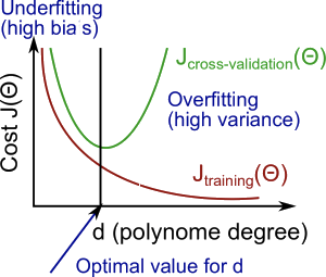
If you run a learning algorithm and it doesn't do as long as you are hoping, almost all the time, it will be because you have either a high bias problem or a high variance problem, in other words, either an underfitting problem or an overfitting problem. In this case, it's very important to figure out which of these two problems is bias or variance or a bit of both that you actually have. Because knowing which of these two things is happening would give a very strong indicator for whether the useful and promising ways to try to improve your algorithm. In this video, I'd like to delve more deeply into this bias and variance issue and understand them better as was figure out how to look in a learning algorithm and evaluate or diagnose whether we might have a bias problem or a variance problem since this will be critical to figuring out how to improve the performance of a learning algorithm that you will implement. So, you've already seen this figure a few times where if you fit two simple hypothesis like a straight line that underfits the data, if you fit a two complex hypothesis, then that might fit the training set perfectly but overfit the data and this may be hypothesis of some intermediate level of complexities of some maybe degree two polynomials or not too low and not too high degree that's like just right and gives you the best generalization error over these options. Now that we're armed with the notion of chain training and validation in test sets, we can understand the concepts of bias and variance a little bit better. Concretely, let's let our training error and cross validation error be defined as in the previous videos. Just say the squared error, the average squared error, as measured on the training sets or as measured on the cross validation set. Now, let's plot the following figure. On the horizontal axis I'm going to plot the degree of polynomial. So, as I go to the right I'm going to be fitting higher and higher order polynomials. So where the left of this figure where maybe d equals one, we're going to be fitting very simple functions whereas we're here on the right of the horizontal axis, I have much larger values of ds, of a much higher degree polynomial. So here, that's going to correspond to fitting much more complex functions to your training set. Let's look at the training error and the cross validation error and plot them on this figure. Let's start with the training error. As we increase the degree of the polynomial, we're going to be able to fit our training set better and better and so if d equals one, then there is high training error, if we have a very high degree of polynomial our training error is going to be really low, maybe even 0 because will fit the training set really well. So, as we increase the degree of polynomial, we find typically that the training error decreases. So I'm going to write J subscript train of theta there, because our training error tends to decrease with the degree of the polynomial that we fit to the data. Next, let's look at the cross-validation error or for that matter, if we look at the test set error, we'll get a pretty similar result as if we were to plot the cross validation error. So, we know that if d equals one, we're fitting a very simple function and so we may be underfitting the training set and so it's going to be very high cross-validation error. If we fit an intermediate degree polynomial, we had d equals two in our example in the previous slide, we're going to have a much lower cross-validation error because we're finding a much better fit to the data. Conversely, if d were too high. So if d took on say a value of four, then we're again overfitting, and so we end up with a high value for cross-validation error. So, if you were to vary this smoothly and plot a curve, you might end up with a curve like that where that's JCV of theta. Again, if you plot J test of theta you get something very similar. So, this sort of plot also helps us to better understand the notions of bias and variance. Concretely, suppose you have applied a learning algorithm and it's not performing as well as you are hoping, so if your cross-validation set error or your test set error is high, how can we figure out if the learning algorithm is suffering from high bias or suffering from high variance? So, the setting of a cross-validation error being high corresponds to either this regime or this regime. So, this regime on the left corresponds to a high bias problem. That is, if you are fitting a overly low order polynomial such as a d equals one when we really needed a higher order polynomial to fit to data, whereas in contrast this regime corresponds to a high variance problem. That is, if d the degree of polynomial was too large for the data set that we have, and this figure gives us a clue for how to distinguish between these two cases. Concretely, for the high bias case, that is the case of underfitting, what we find is that both the cross validation error and the training error are going to be high. So, if your algorithm is suffering from a bias problem, the training set error will be high and you might find that the cross validation error will also be high. It might be close, maybe just slightly higher, than the training error. So, if you see this combination, that's a sign that your algorithm may be suffering from high bias. In contrast, if your algorithm is suffering from high variance, then if you look here, we'll notice that J train, that is the training error, is going to be low. That is, you're fitting the training set very well, whereas your cross validation error assuming that this is, say, the squared error which we're trying to minimize say, whereas in contrast your error on a cross validation set or your cross function or cross validation set will be much bigger than your training set error. So, this is a double greater than sign. That's the map symbol for much greater thans, denoted by two greater than signs. So if you see this combination of values, then that's a clue that your learning algorithm may be suffering from high variance and might be overfitting. The key that distinguishes these two cases is, if you have a high bias problem, your training set error will also be high is your hypothesis just not fitting the training set well. If you have a high variance problem, your training set error will usually be low, that is much lower than your cross-validation error. So hopefully that gives you a somewhat better understanding of the two problems of bias and variance. I still have a lot more to say about bias and variance in the next few videos, but what we'll see later is that by diagnosing whether a learning algorithm may be suffering from high bias or high variance, I'll show you even more details on how to do that in later videos. But we'll see that by figuring out whether a learning algorithm may be suffering from high bias or high variance or combination of both, that that would give us much better guidance for what might be promising things to try in order to improve the performance of a learning algorithm.
Reading: Diagnosing Bias vs. Variance
Diagnosing Bias vs. Variance
In this section we examine the relationship between the degree of the polynomial d and the underfitting or overfitting of our hypothesis.
- We need to distinguish whether bias or variance is the problem contributing to bad predictions.
- High bias is underfitting and high variance is overfitting. Ideally, we need to find a golden mean between these two.
The training error will tend to decrease as we increase the degree d of the polynomial.
At the same time, the cross validation error will tend to decrease as we increase d up to a point, and then it will increase as d is increased, forming a convex curve.
High bias (underfitting): both (J_{train}(Theta)) and (J_{CV}(Theta)) will be high. Also, (J_{CV}(Theta) approx J_{train}(Theta)).
High variance (overfitting): (J_{train}(Theta)) will be low and (J_{CV}(Theta)) will be much greater than (J_{train}(Theta)).
The is summarized in the figure below:
Video: Regularization and Bias/Variance
You've seen how regularization can help prevent over-fitting. But how does it affect the bias and variances of a learning algorithm? In this video I'd like to go deeper into the issue of bias and variances and talk about how it interacts with and is affected by the regularization of your learning algorithm.
0:22
Suppose we're fitting a high auto polynomial, like that showed here, but to prevent over fitting we need to use regularization, like that shown here. So we have this regularization term to try to keep the values of the prem to small. And as usual, the regularizations comes from J = 1 to m, rather than j = 0 to m. Let's consider three cases. The first is the case of the very large value of the regularization parameter lambda, such as if lambda were equal to 10,000. Some huge value.
0:54
In this case, all of these parameters, theta 1, theta 2, theta 3, and so on would be heavily penalized and so we end up with most of these parameter values being closer to zero. And the hypothesis will be roughly h of x, just equal or approximately equal to theta zero. So we end up with a hypothesis that more or less looks like that, more or less a flat, constant straight line. And so this hypothesis has high bias and it badly under fits this data set, so the horizontal straight line is just not a very good model for this data set. At the other extreme is if we have a very small value of lambda, such as if lambda were equal to zero. In that case, given that we're fitting a high order polynomial, this is a usual over-fitting setting. In that case, given that we're fitting a high-order polynomial, basically, without regularization or with very minimal regularization, we end up with our usual high-variance, over fitting setting. This is basically if lambda is equal to zero, we're just fitting with our regularization, so that over fits the hypothesis. And it's only if we have some intermediate value of longer that is neither too large nor too small that we end up with parameters data that give us a reasonable fit to this data. So, how can we automatically choose a good value for the regularization parameter?
2:19
Just to reiterate, here's our model, and here's our learning algorithm's objective. For the setting where we're using regularization, let me define J train(theta) to be something different, to be the optimization objective, but without the regularization term. Previously, in an earlier video, when we were not using regularization I define J train of data to be the same as J of theta as the cause function but when we're using regularization when the six well under term we're going to define J train my training set to be just my sum of squared errors on the training set or my average squared error on the training set without taking into account that regularization. And similarly I'm then also going to define the cross validation sets error and to test that error as before to be the average sum of squared errors on the cross validation in the test sets so just to summarize my definitions of J train J CU and J test are just the average square there one half of the other square record on the training validation of the test set without the extra regularization term. So, this is how we can automatically choose the regularization parameter lambda. So what I usually do is maybe have some range of values of lambda I want to try out. So I might be considering not using regularization or here are a few values I might try lambda considering lambda = 0.01, 0.02, 0.04, and so on. And I usually set these up in multiples of two, until some maybe larger value if I were to do these in multiples of 2 I'd end up with a 10.24. It's 10 exactly, but this is close enough. And the three to four decimal places won't effect your result that much. So, this gives me maybe 12 different models. And I'm trying to select a month corresponding to 12 different values of the regularization of the parameter lambda. And of course you can also go to values less than 0.01 or values larger than 10 but I've just truncated it here for convenience. Given the issue of these 12 models, what we can do is then the following, we can take this first model with lambda equals zero and minimize my cost function J of data and this will give me some parameter of active data. And similar to the earlier video, let me just denote this as theta super script one.
4:49
And then I can take my second model with lambda set to 0.01 and minimize my cost function now using lambda equals 0.01 of course. To get some different parameter vector theta. Let me denote that theta(2). And for that I end up with theta(3). So if part for my third model. And so on until for my final model with lambda set to 10 or 10.24, I end up with this theta(12). Next, I can talk all of these hypotheses, all of these parameters and use my cross validation set to validate them so I can look at my first model, my second model, fit to these different values of the regularization parameter, and evaluate them with my cross validation set based in measure the average square error of each of these square vector parameters theta on my cross validation sets. And I would then pick whichever one of these 12 models gives me the lowest error on the trans validation set. And let's say, for the sake of this example, that I end up picking theta 5, the 5th order polynomial, because that has the lowest cause validation error. Having done that, finally what I would do if I wanted to report each test set error, is to take the parameter theta 5 that I've selected, and look at how well it does on my test set. So once again, here is as if we've fit this parameter, theta, to my cross-validation set, which is why I'm setting aside a separate test set that I'm going to use to get a better estimate of how well my parameter vector, theta, will generalize to previously unseen examples. So that's model selection applied to selecting the regularization parameter lambda. The last thing I'd like to do in this video is get a better understanding of how cross validation and training error vary as we vary the regularization parameter lambda. And so just a reminder right, that was our original cost on j of theta. But for this purpose we're going to define training error without using a regularization parameter, and cross validation error without using the regularization parameter.
7:07
And what I'd like to do is plot this Jtrain and plot this Jcv, meaning just how well does my hypothesis do on the training set and how does my hypothesis do when it cross validation sets. As I vary my regularization parameter lambda.
7:27
So as we saw earlier if lambda is small then we're not using much regularization
7:35
and we run a larger risk of over fitting whereas if lambda is large that is if we were on the right part of this horizontal axis then, with a large value of lambda, we run the higher risk of having a biased problem, so if you plot J train and J cv, what you find is that, for small values of lambda, you can fit the trading set relatively way cuz you're not regularizing. So, for small values of lambda, the regularization term basically goes away, and you're just minimizing pretty much just gray arrows. So when lambda is small, you end up with a small value for Jtrain, whereas if lambda is large, then you have a high bias problem, and you might not feel your training that well, so you end up the value up there. So Jtrain of theta will tend to increase when lambda increases, because a large value of lambda corresponds to high bias where you might not even fit your trainings that well, whereas a small value of lambda corresponds to, if you can really fit a very high degree polynomial to your data, let's say. After the cost validation error we end up with a figure like this,
8:51
where over here on the right, if we have a large value of lambda, we may end up under fitting, and so this is the bias regime. And so the cross validation error will be high. Let me just leave all of that to this Jcv (theta) because so, with high bias, we won't be fitting, we won't be doing well in cross validation sets, whereas here on the left, this is the high variance regime, where we have two smaller value with longer, then we may be over fitting the data. And so by over fitting the data, then the cross validation error will also be high. And so, this is what the cross validation error and what the trading error may look like on a trading stance as we vary the regularization parameter lambda. And so once again, it will often be some intermediate value of lambda that is just right or that works best In terms of having a small cross validation error or a small test theta. And whereas the curves I've drawn here are somewhat cartoonish and somewhat idealized so on the real data set the curves you get may end up looking a little bit more messy and just a little bit more noisy then this. For some data sets you will really see these for sorts of trends and by looking at a plot of the hold-out cross validation error you can either manual, automatically try to select a point that minimizes the cross validation error and select the value of lambda corresponding to low cross validation error. When I'm trying to pick the regularization parameter lambda for learning algorithm, often I find that plotting a figure like this one shown here helps me understand better what's going on and helps me verify that I am indeed picking a good value for the regularization parameter monitor. So hopefully that gives you more insight into regularization and it's effects on the bias and variance of a learning algorithm. By now you've seen bias and variance from a lot of different perspectives. And what we like to do in the next video is take all the insights we've gone through and build on them to put together a diagnostic that's called learning curves, which is a tool that I often use to diagnose if the learning algorithm may be suffering from a bias problem or a variance problem, or a little bit of both.
Reading: Regularization and Bias/Variance
Regularization and Bias/Variance
Note: [The regularization term below and through out the video should be (frac lambda {2m} sum _{j=1}^n heta_j ^2) and NOT (frac lambda {2m} sum _{j=1}^m heta_j ^2)]
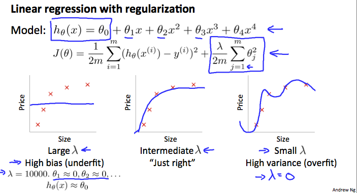
In the figure above, we see that as (lambda) increases, our fit becomes more rigid. On the other hand, as (lambda) approaches 0, we tend to over overfit the data. So how do we choose our parameter (lambda) to get it 'just right' ? In order to choose the model and the regularization term λ, we need to:
- Create a list of lambdas (i.e. λ∈{0,0.01,0.02,0.04,0.08,0.16,0.32,0.64,1.28,2.56,5.12,10.24});
- Create a set of models with different degrees or any other variants.
- Iterate through the (lambda)s and for each (lambda) go through all the models to learn some (Theta).
- Compute the cross validation error using the learned Θ (computed with λ) on the (J_{CV}(Theta)) without regularization or λ = 0.
- Select the best combo that produces the lowest error on the cross validation set.
- Using the best combo Θ and λ, apply it on (J_{test}(Theta)) to see if it has a good generalization of the problem.
Video: Learning Curves
In this video, I'd like to tell you about learning curves.
0:03
Learning curves is often a very useful thing to plot. If either you wanted to sanity check that your algorithm is working correctly, or if you want to improve the performance of the algorithm.
0:13
And learning curves is a tool that I actually use very often to try to diagnose if a physical learning algorithm may be suffering from bias, sort of variance problem or a bit of both.
0:27
Here's what a learning curve is. To plot a learning curve, what I usually do is plot j train which is, say,
0:35
average squared error on my training set or Jcv which is the average squared error on my cross validation set. And I'm going to plot that as a function of m, that is as a function of the number of training examples I have. And so m is usually a constant like maybe I just have, you know, a 100 training examples but what I'm going to do is artificially with use my training set exercise. So, I deliberately limit myself to using only, say, 10 or 20 or 30 or 40 training examples and plot what the training error is and what the cross validation is for this smallest training set exercises. So let's see what these plots may look like. Suppose I have only one training example like that shown in this this first example here and let's say I'm fitting a quadratic function. Well, I
1:22
have only one training example. I'm going to be able to fit it perfectly right? You know, just fit the quadratic function. I'm going to have 0 error on the one training example. If I have two training examples. Well the quadratic function can also fit that very well. So,
1:37
even if I am using regularization, I can probably fit this quite well. And if I am using no neural regularization, I'm going to fit this perfectly and if I have three training examples again. Yeah, I can fit a quadratic function perfectly so if m equals 1 or m equals 2 or m equals 3,
1:54
my training error on my training set is going to be 0 assuming I'm not using regularization or it may slightly large in 0 if I'm using regularization and by the way if I have a large training set and I'm artificially restricting the size of my training set in order to J train. Here if I set M equals 3, say, and I train on only three examples, then, for this figure I am going to measure my training error only on the three examples that actually fit my data too
2:27
and so even I have to say a 100 training examples but if I want to plot what my training error is the m equals 3. What I'm going to do
2:34
is to measure the training error on the three examples that I've actually fit to my hypothesis 2.
2:41
And not all the other examples that I have deliberately omitted from the training process. So just to summarize what we've seen is that if the training set size is small then the training error is going to be small as well. Because you know, we have a small training set is going to be very easy to fit your training set very well may be even perfectly now say we have m equals 4 for example. Well then a quadratic function can be a longer fit this data set perfectly and if I have m equals 5 then you know, maybe quadratic function will fit to stay there so so, then as my training set gets larger.
3:16
It becomes harder and harder to ensure that I can find the quadratic function that process through all my examples perfectly. So in fact as the training set size grows what you find is that my average training error actually increases and so if you plot this figure what you find is that the training set error that is the average error on your hypothesis grows as m grows and just to repeat when the intuition is that when m is small when you have very few training examples. It's pretty easy to fit every single one of your training examples perfectly and so your error is going to be small whereas when m is larger then gets harder all the training examples perfectly and so your training set error becomes more larger now, how about the cross validation error. Well, the cross validation is my error on this cross validation set that I haven't seen and so, you know, when I have a very small training set, I'm not going to generalize well, just not going to do well on that. So, right, this hypothesis here doesn't look like a good one, and it's only when I get a larger training set that, you know, I'm starting to get hypotheses that maybe fit the data somewhat better. So your cross validation error and your test set error will tend to decrease as your training set size increases because the more data you have, the better you do at generalizing to new examples. So, just the more data you have, the better the hypothesis you fit. So if you plot j train, and Jcv this is the sort of thing that you get. Now let's look at what the learning curves may look like if we have either high bias or high variance problems. Suppose your hypothesis has high bias and to explain this I'm going to use a, set an example, of fitting a straight line to data that, you know, can't really be fit well by a straight line.
5:09
So we end up with a hypotheses that maybe looks like that.
5:13
Now let's think what would happen if we were to increase the training set size. So if instead of five examples like what I've drawn there, imagine that we have a lot more training examples.
5:25
Well what happens, if you fit a straight line to this. What you find is that, you end up with you know, pretty much the same straight line. I mean a straight line that just cannot fit this data and getting a ton more data, well the straight line isn't going to change that much. This is the best possible straight-line fit to this data, but the straight line just can't fit this data set that well. So, if you plot across validation error,
5:49
this is what it will look like.
5:51
Option on the left, if you have already a miniscule training set size like you know, maybe just one training example and is not going to do well. But by the time you have reached a certain number of training examples, you have almost fit the best possible straight line, and even if you end up with a much larger training set size, a much larger value of m, you know, you're basically getting the same straight line, and so, the cross-validation error - let me label that - or test set error or plateau out, or flatten out pretty soon, once you reached beyond a certain the number of training examples, unless you pretty much fit the best possible straight line. And how about training error? Well, the training error will again be small.
6:34
And what you find in the high bias case is that the training error will end up close to the cross validation error, because you have so few parameters and so much data, at least when m is large. The performance on the training set and the cross validation set will be very similar.
6:53
And so, this is what your learning curves will look like, if you have an algorithm that has high bias.
7:00
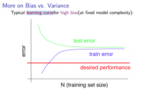
And finally, the problem with high bias is reflected in the fact that both the cross validation error and the training error are high, and so you end up with a relatively high value of both Jcv and the j train.
7:15
This also implies something very interesting, which is that, if a learning algorithm has high bias, as we get more and more training examples, that is, as we move to the right of this figure, we'll notice that the cross validation error isn't going down much, it's basically fattened up, and so if learning algorithms are really suffering from high bias.
7:36
Getting more training data by itself will actually not help that much,and as our figure example in the figure on the right, here we had only five training. examples, and we fill certain straight line. And when we had a ton more training data, we still end up with roughly the same straight line. And so if the learning algorithm has high bias give me a lot more training data. That doesn't actually help you get a much lower cross validation error or test set error. So knowing if your learning algorithm is suffering from high bias seems like a useful thing to know because this can prevent you from wasting a lot of time collecting more training data where it might just not end up being helpful. Next let us look at the setting of a learning algorithm that may have high variance.
8:21
Let us just look at the training error in a around if you have very smart training set like five training examples shown on the figure on the right and if we're fitting say a very high order polynomial,
8:34
and I've written a hundredth degree polynomial which really no one uses, but just an illustration.
8:39
And if we're using a fairly small value of lambda, maybe not zero, but a fairly small value of lambda, then we'll end up, you know, fitting this data very well that with a function that overfits this. So, if the training set size is small, our training error, that is, j train of theta will be small.
9:03
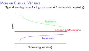
And as this training set size increases a bit, you know, we may still be overfitting this data a little bit but it also becomes slightly harder to fit this data set perfectly, and so, as the training set size increases, we'll find that j train increases, because it is just a little harder to fit the training set perfectly when we have more examples, but the training set error will still be pretty low. Now, how about the cross validation error? Well, in high variance setting, a hypothesis is overfitting and so the cross validation error will remain high, even as we get you know, a moderate number of training examples and, so maybe, the cross validation error may look like that. And the indicative diagnostic that we have a high variance problem,
9:50
is the fact that there's this large gap between the training error and the cross validation error.
9:57
And looking at this figure. If we think about adding more training data, that is, taking this figure and extrapolating to the right, we can kind of tell that, you know the two curves, the blue curve and the magenta curve, are converging to each other. And so, if we were to extrapolate this figure to the right, then it seems it likely that the training error will keep on going up and the
10:27
cross-validation error would keep on going down. And the thing we really care about is the cross-validation error or the test set error, right? So in this sort of figure, we can tell that if we keep on adding training examples and extrapolate to the right, well our cross validation error will keep on coming down. And, so, in the high variance setting, getting more training data is, indeed, likely to help. And so again, this seems like a useful thing to know if your learning algorithm is suffering from a high variance problem, because that tells you, for example that it may be be worth your while to see if you can go and get some more training data.
11:03
Now, on the previous slide and this slide, I've drawn fairly clean fairly idealized curves. If you plot these curves for an actual learning algorithm, sometimes you will actually see, you know, pretty much curves, like what I've drawn here. Although, sometimes you see curves that are a little bit noisier and a little bit messier than this. But plotting learning curves like these can often tell you, can often help you figure out if your learning algorithm is suffering from bias, or variance or even a little bit of both. So when I'm trying to improve the performance of a learning algorithm, one thing that I'll almost always do is plot these learning curves, and usually this will give you a better sense of whether there is a bias or variance problem.
11:44
And in the next video we'll see how this can help suggest specific actions is to take, or to not take, in order to try to improve the performance of your learning algorithm.
Reading: Learning Curves
Learning Curves
Training an algorithm on a very few number of data points (such as 1, 2 or 3) will easily have 0 errors because we can always find a quadratic curve that touches exactly those number of points. Hence:
- As the training set gets larger, the error for a quadratic function increases.
- The error value will plateau out after a certain m, or training set size.
Experiencing high bias:
Low training set size: causes (J_{train}(Theta)) to be low and (J_{CV}(Theta)) to be high.
Large training set size: causes both (J_{train}(Theta)) and (J_{CV}(Theta)) to be high with (J_{train}(Theta)≈J_{CV}(Theta)).
If a learning algorithm is suffering from high bias, getting more training data will not (by itself) help much.
Experiencing high variance:
Low training set size: (J_{train}(Theta)) will be low and (J_{CV}(Theta)) will be high.
Large training set size: (J_{train}(Theta)) increases with training set size and (J_{CV}(Theta)) continues to decrease without leveling off. Also, (J_{train}(Theta) < J_{CV}(Theta)) but the difference between them remains significant.
If a learning algorithm is suffering from high variance, getting more training data is likely to help.
Video: Deciding What to Do Next Revisited
We've talked about how to evaluate learning algorithms, talked about model selection, talked a lot about bias and variance. So how does this help us figure out what are potentially fruitful, potentially not fruitful things to try to do to improve the performance of a learning algorithm.
0:15
Let's go back to our original motivating example and go for the result.
0:21
So here is our earlier example of maybe having fit regularized linear regression and finding that it doesn't work as well as we're hoping. We said that we had this menu of options. So is there some way to figure out which of these might be fruitful options? The first thing all of this was getting more training examples. What this is good for, is this helps to fix high variance.
0:45
And concretely, if you instead have a high bias problem and don't have any variance problem, then we saw in the previous video that getting more training examples,
0:54
while maybe just isn't going to help much at all. So the first option is useful only if you, say, plot the learning curves and figure out that you have at least a bit of a variance, meaning that the cross-validation error is, you know, quite a bit bigger than your training set error. How about trying a smaller set of features? Well, trying a smaller set of features, that's again something that fixes high variance.
1:17
And in other words, if you figure out, by looking at learning curves or something else that you used, that have a high bias problem; then for goodness sakes, don't waste your time trying to carefully select out a smaller set of features to use. Because if you have a high bias problem, using fewer features is not going to help. Whereas in contrast, if you look at the learning curves or something else you figure out that you have a high variance problem, then, indeed trying to select out a smaller set of features, that might indeed be a very good use of your time. How about trying to get additional features, adding features, usually, not always, but usually we think of this as a solution
1:54
for fixing high bias problems. So if you are adding extra features it's usually because
2:01
your current hypothesis is too simple, and so we want to try to get additional features to make our hypothesis better able to fit the training set. And similarly, adding polynomial features; this is another way of adding features and so there is another way to try to fix the high bias problem.
2:21
And, if concretely if your learning curves show you that you still have a high variance problem, then, you know, again this is maybe a less good use of your time.
2:30
And finally, decreasing and increasing lambda. This are quick and easy to try, I guess these are less likely to be a waste of, you know, many months of your life. But decreasing lambda, you already know fixes high bias.
2:45
In case this isn't clear to you, you know, I do encourage you to pause the video and think through this that convince yourself that decreasing lambda helps fix high bias, whereas increasing lambda fixes high variance.
2:59
And if you aren't sure why this is the case, do pause the video and make sure you can convince yourself that this is the case. Or take a look at the curves that we were plotting at the end of the previous video and try to make sure you understand why these are the case.
3:15
Finally, let us take everything we have learned and relate it back to neural networks and so, here is some practical advice for how I usually choose the architecture or the connectivity pattern of the neural networks I use.
3:30
So, if you are fitting a neural network, one option would be to fit, say, a pretty small neural network with you know, relatively few hidden units, maybe just one hidden unit. If you're fitting a neural network, one option would be to fit a relatively small neural network with, say,
3:48
relatively few, maybe only one hidden layer and maybe only a relatively few number of hidden units. So, a network like this might have relatively few parameters and be more prone to underfitting.
4:00
The main advantage of these small neural networks is that the computation will be cheaper.
4:05
An alternative would be to fit a, maybe relatively large neural network with either more hidden units--there's a lot of hidden in one there--or with more hidden layers.
4:16
And so these neural networks tend to have more parameters and therefore be more prone to overfitting.
4:22
One disadvantage, often not a major one but something to think about, is that if you have a large number of neurons in your network, then it can be more computationally expensive.
4:33
Although within reason, this is often hopefully not a huge problem.
4:36
The main potential problem of these much larger neural networks is that it could be more prone to overfitting and it turns out if you're applying neural network very often using a large neural network often it's actually the larger, the better
4:50
but if it's overfitting, you can then use regularization to address overfitting, usually using a larger neural network by using regularization to address is overfitting that's often more effective than using a smaller neural network. And the main possible disadvantage is that it can be more computationally expensive.
5:10
And finally, one of the other decisions is, say, the number of hidden layers you want to have, right? So, do you want one hidden layer or do you want three hidden layers, as we've shown here, or do you want two hidden layers?
5:23
And usually, as I think I said in the previous video, using a single hidden layer is a reasonable default, but if you want to choose the number of hidden layers, one other thing you can try is find yourself a training cross-validation, and test set split and try training neural networks with one hidden layer or two hidden layers or three hidden layers and see which of those neural networks performs best on the cross-validation sets. You take your three neural networks with one, two and three hidden layers, and compute the cross validation error at Jcv and all of them and use that to select which of these is you think the best neural network.
6:02
So, that's it for bias and variance and ways like learning curves, who tried to diagnose these problems. As far as what you think is implied, for one might be truthful or not truthful things to try to improve the performance of a learning algorithm.
6:16
If you understood the contents of the last few videos and if you apply them you actually be much more effective already and getting learning algorithms to work on problems and even a large fraction, maybe the majority of practitioners of machine learning here in Silicon Valley today doing these things as their full-time jobs.
6:35
So I hope that these pieces of advice on by experience in diagnostics
6:42
will help you to much effectively and powerfully apply learning and get them to work very well.
Reading: Deciding What to do Next Revisited
Deciding What to Do Next Revisited
Our decision process can be broken down as follows:
- Getting more training examples: Fixes high variance
- Trying smaller sets of features: Fixes high variance
- Adding features: Fixes high bias
- Adding polynomial features: Fixes high bias
- Decreasing λ: Fixes high bias
- Increasing λ: Fixes high variance.
Diagnosing Neural Networks
- A neural network with fewer parameters is prone to underfitting. It is also computationally cheaper.
- A large neural network with more parameters is prone to overfitting. It is also computationally expensive. In this case you can use regularization (increase λ) to address the overfitting.
Using a single hidden layer is a good starting default. You can train your neural network on a number of hidden layers using your cross validation set. You can then select the one that performs best.
Model Complexity Effects:
- Lower-order polynomials (low model complexity) have high bias and low variance. In this case, the model fits poorly consistently.
- Higher-order polynomials (high model complexity) fit the training data extremely well and the test data extremely poorly. These have low bias on the training data, but very high variance.
- In reality, we would want to choose a model somewhere in between, that can generalize well but also fits the data reasonably well.
Reading: Lecture Slides
Programming: Regularized Linear Regression and Bias/Variance
Download the programming assignment here. This ZIP file contains the instructions in a PDF and the starter code. You may use either MATLAB or Octave (>= 3.8.0).
Machine Learning System Design
To optimize a machine learning algorithm, you’ll need to first understand where the biggest improvements can be made. In this module, we discuss how to understand the performance of a machine learning system with multiple parts, and also how to deal with skewed data.
5 videos, 3 readings
Video: Prioritizing What to Work On
In the next few videos I'd like to talk about machine learning system design.
0:05
These videos will touch on the main issues that you may face when designing a complex machine learning system,
0:12
and will actually try to give advice on how to strategize putting together a complex machine learning system.
0:18
In case this next set of videos seems a little disjointed that's because these videos will touch on a range of the different issues that you may come across when designing complex learning systems.
0:29
And even though the next set of videos may seem somewhat less mathematical, I think that this material may turn out to be very useful, and potentially huge time savers when you're building big machine learning systems.
0:42
Concretely, I'd like to begin with the issue of prioritizing how to spend your time on what to work on, and I'll begin with an example on spam classification.
0:55
Let's say you want to build a spam classifier.
0:58
Here are a couple of examples of obvious spam and non-spam emails.
1:03
if the one on the left tried to sell things. And notice how spammers will deliberately misspell words, like Vincent with a 1 there, and mortgages.
1:14
And on the right as maybe an obvious example of non-stamp email, actually email from my younger brother.
1:21
Let's say we have a labeled training set of some number of spam emails and some non-spam emails denoted with labels y equals 1 or 0, how do we build a classifier using supervised learning to distinguish between spam and non-spam?
1:38
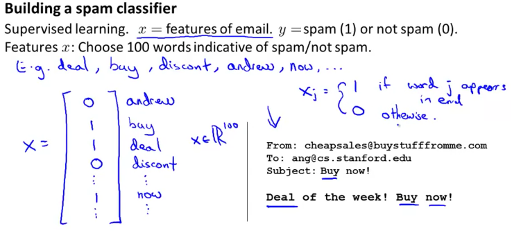
In order to apply supervised learning, the first decision we must make is how do we want to represent x, that is the features of the email. Given the features x and the labels y in our training set, we can then train a classifier, for example using logistic regression.
1:56
Here's one way to choose a set of features for our emails.
2:00
We could come up with, say, a list of maybe a hundred words that we think are indicative of whether e-mail is spam or non-spam, for example, if a piece of e-mail contains the word 'deal' maybe it's more likely to be spam if it contains the word 'buy' maybe more likely to be spam, a word like 'discount' is more likely to be spam, whereas if a piece of email contains my name,
2:23
Andrew, maybe that means the person actually knows who I am and that might mean it's less likely to be spam.
2:31
And maybe for some reason I think the word "now" may be indicative of non-spam because I get a lot of urgent emails, and so on, and maybe we choose a hundred words or so.
2:42
Given a piece of email, we can then take this piece of email and encode it into a feature vector as follows. I'm going to take my list of a hundred words and sort them in alphabetical order say. It doesn't have to be sorted. But, you know, here's a, here's my list of words, just count and so on, until eventually I'll get down to now, and so on and given a piece of e-mail like that shown on the right, I'm going to check and see whether or not each of these words appears in the e-mail and then I'm going to define a feature vector x where in this piece of an email on the right, my name doesn't appear so I'm gonna put a zero there. The word "by" does appear,
3:26
so I'm gonna put a one there and I'm just gonna put one's or zeroes. I'm gonna put a one even though the word "by" occurs twice. I'm not gonna recount how many times the word occurs.
3:37
The word "due" appears, I put a one there. The word "discount" doesn't appear, at least not in this this little short email, and so on. The word "now" does appear and so on. So I put ones and zeroes in this feature vector depending on whether or not a particular word appears. And in this example my feature vector would have to mention one hundred,
4:02
if I have a hundred, if if I chose a hundred words to use for this representation and each of my features Xj will basically be 1 if
4:16
you have a particular word that, we'll call this word j, appears in the email and Xj
4:22
would be zero otherwise.
4:25
Okay. So that gives me a feature representation of a piece of email. By the way, even though I've described this process as manually picking a hundred words, in practice what's most commonly done is to look through a training set, and in the training set depict the most frequently occurring n words where n is usually between ten thousand and fifty thousand, and use those as your features. So rather than manually picking a hundred words, here you look through the training examples and pick the most frequently occurring words like ten thousand to fifty thousand words, and those form the features that you are going to use to represent your email for spam classification.
5:05
Now, if you're building a spam classifier one question that you may face is, what's the best use of your time in order to make your spam classifier have higher accuracy, you have lower error.
5:18
One natural inclination is going to collect lots of data. Right? And in fact there's this tendency to think that, well the more data we have the better the algorithm will do. And in fact, in the email spam domain, there are actually pretty serious projects called Honey Pot Projects, which create fake email addresses and try to get these fake email addresses into the hands of spammers and use that to try to collect tons of spam email, and therefore you know, get a lot of spam data to train learning algorithms. But we've already seen in the previous sets of videos that getting lots of data will often help, but not all the time.
5:54
But for most machine learning problems, there are a lot of other things you could usually imagine doing to improve performance.
6:00
For spam, one thing you might think of is to develop more sophisticated features on the email, maybe based on the email routing information.
6:09
And this would be information contained in the email header.
6:13
So, when spammers send email, very often they will try to obscure the origins of the email, and maybe use fake email headers.
6:22
Or send email through very unusual sets of computer service. Through very unusual routes, in order to get the spam to you. And some of this information will be reflected in the email header.
6:35
And so one can imagine,
6:38
looking at the email headers and trying to develop more sophisticated features to capture this sort of email routing information to identify if something is spam. Something else you might consider doing is to look at the email message body, that is the email text, and try to develop more sophisticated features. For example, should the word 'discount' and the word 'discounts' be treated as the same words or should we have treat the words 'deal' and 'dealer' as the same word? Maybe even though one is lower case and one in capitalized in this example. Or do we want more complex features about punctuation because maybe spam
7:12
is using exclamation marks a lot more. I don't know. And along the same lines, maybe we also want to develop more sophisticated algorithms to detect and maybe to correct to deliberate misspellings, like mortgage, medicine, watches.
7:25
Because spammers actually do this, because if you have watches
7:29
with a 4 in there then well, with the simple technique that we talked about just now, the spam classifier might not equate this as the same thing as the word "watches," and so it may have a harder time realizing that something is spam with these deliberate misspellings. And this is why spammers do it.
7:48
While working on a machine learning problem, very often you can brainstorm lists of different things to try, like these. By the way, I've actually worked on the spam problem myself for a while. And I actually spent quite some time on it. And even though I kind of understand the spam problem, I actually know a bit about it, I would actually have a very hard time telling you of these four options which is the best use of your time so what happens, frankly what happens far too often is that a research group or product group will randomly fixate on one of these options. And sometimes that turns out not to be the most fruitful way to spend your time depending, you know, on which of these options someone ends up randomly fixating on. By the way, in fact, if you even get to the stage where you brainstorm a list of different options to try, you're probably already ahead of the curve. Sadly, what most people do is instead of trying to list out the options of things you might try, what far too many people do is wake up one morning and, for some reason, just, you know, have a weird gut feeling that, "Oh let's have a huge honeypot project to go and collect tons more data" and for whatever strange reason just sort of wake up one morning and randomly fixate on one thing and just work on that for six months.
9:03
But I think we can do better. And in particular what I'd like to do in the next video is tell you about the concept of error analysis
9:11
and talk about the way where you can try to have a more systematic way to choose amongst the options of the many different things you might work, and therefore be more likely to select what is actually a good way to spend your time, you know for the next few weeks, or next few days or the next few months.
Reading: Prioritizing What to Work On
Prioritizing What to Work On
System Design Example:
Given a data set of emails, we could construct a vector for each email. Each entry in this vector represents a word. The vector normally contains 10,000 to 50,000 entries gathered by finding the most frequently used words in our data set. If a word is to be found in the email, we would assign its respective entry a 1, else if it is not found, that entry would be a 0. Once we have all our x vectors ready, we train our algorithm and finally, we could use it to classify if an email is a spam or not.
So how could you spend your time to improve the accuracy of this classifier?
- Collect lots of data (for example "honeypot" project but doesn't always work)
- Develop sophisticated features (for example: using email header data in spam emails)
- Develop algorithms to process your input in different ways (recognizing misspellings in spam).
It is difficult to tell which of the options will be most helpful.
Video: Error Analysis
In the last video I talked about how, when faced with a machine learning problem, there are often lots of different ideas for how to improve the algorithm. In this video, let's talk about the concept of error analysis. Which will hopefully give you a way to more systematically make some of these decisions.
0:17
If you're starting work on a machine learning problem, or building a machine learning application. It's often considered very good practice to start, not by building a very complicated system with lots of complex features and so on. But to instead start by building a very simple algorithm that you can implement quickly. And when I start with a learning problem what I usually do is spend at most one day, like literally at most 24 hours, To try to get something really quick and dirty. Frankly not at all sophisticated system but get something really quick and dirty running, and implement it and then test it on my cross-validation data. Once you've done that you can then plot learning curves, this is what we talked about in the previous set of videos. But plot learning curves of the training and test errors to try to figure out if you're learning algorithm maybe suffering from high bias or high variance, or something else. And use that to try to decide if having more data, more features, and so on are likely to help. And the reason that this is a good approach is often, when you're just starting out on a learning problem, there's really no way to tell in advance. Whether you need more complex features, or whether you need more data, or something else. And it's just very hard to tell in advance, that is, in the absence of evidence, in the absence of seeing a learning curve. It's just incredibly difficult to figure out where you should be spending your time. And it's often by implementing even a very, very quick and dirty implementation. And by plotting learning curves, that helps you make these decisions. So if you like you can to think of this as a way of avoiding whats sometimes called premature optimization in computer programming. And this idea that says we should let evidence guide our decisions on where to spend our time rather than use gut feeling, which is often wrong. In addition to plotting learning curves, one other thing that's often very useful to do is what's called error analysis. And what I mean by that is that when building say a spam classifier. I will often look at my cross validation set and manually look at the emails that my algorithm is making errors on. So look at the spam e-mails and non-spam e-mails that the algorithm is misclassifying and see if you can spot any systematic patterns in what type of examples it is misclassifying. And often, by doing that, this is the process that will inspire you to design new features. Or they'll tell you what are the current things or current shortcomings of the system. And give you the inspiration you need to come up with improvements to it. Concretely, here's a specific example. Let's say you've built a spam classifier and you have 500 examples in your cross validation set. And let's say in this example that the algorithm has a very high error rate. And this classifies 100 of these cross validation examples.
3:18
So what I do is manually examine these 100 errors and manually categorize them. Based on things like what type of email it is, what cues or what features you think might have helped the algorithm classify them correctly. So, specifically, by what type of email it is, if I look through these 100 errors, I might find that maybe the most common types of spam emails in these classifies are maybe emails on pharma or pharmacies, trying to sell drugs. Maybe emails that are trying to sell replicas such as fake watches, fake random things, maybe some emails trying to steal passwords,. These are also called phishing emails, that's another big category of emails, and maybe other categories. So in terms of classify what type of email it is, I would actually go through and count up my hundred emails. Maybe I find that 12 of them is label emails, or pharma emails, and maybe 4 of them are emails trying to sell replicas, that sell fake watches or something. And maybe I find that 53 of them are these what's called phishing emails, basically emails trying to persuade you to give them your password. And 31 emails are other types of emails. And it's by counting up the number of emails in these different categories that you might discover, for example. That the algorithm is doing really, particularly poorly on emails trying to steal passwords. And that may suggest that it might be worth your effort to look more carefully at that type of email and see if you can come up with better features to categorize them correctly.
4:57
And, also what I might do is look at what cues or what additional features might have helped the algorithm classify the emails. So let's say that some of our hypotheses about things or features that might help us classify emails better are. Trying to detect deliberate misspellings versus unusual email routing versus unusual spamming punctuation. Such as if people use a lot of exclamation marks. And once again I would manually go through and let's say I find five cases of this and 16 of this and 32 of this and a bunch of other types of emails as well. And if this is what you get on your cross validation set, then it really tells you that maybe deliberate spellings is a sufficiently rare phenomenon that maybe it's not worth all the time trying to write algorithms that detect that. But if you find that a lot of spammers are using, you know, unusual punctuation, then maybe that's a strong sign that it might actually be worth your while to spend the time to develop more sophisticated features based on the punctuation. So this sort of error analysis, which is really the process of manually examining the mistakes that the algorithm makes, can often help guide you to the most fruitful avenues to pursue. And this also explains why I often recommend implementing a quick and dirty implementation of an algorithm. What we really want to do is figure out what are the most difficult examples for an algorithm to classify. And very often for different algorithms, for different learning algorithms they'll often find similar categories of examples difficult. And by having a quick and dirty implementation, that's often a quick way to let you identify some errors and quickly identify what are the hard examples. So that you can focus your effort on those.
6:49
Lastly, when developing learning algorithms, one other useful tip is to make sure that you have a numerical evaluation of your learning algorithm.
7:01
And what I mean by that is you if you're developing a learning algorithm, it's often incredibly helpful. If you have a way of evaluating your learning algorithm that just gives you back a single real number, maybe accuracy, maybe error. But the single real number that tells you how well your learning algorithm is doing. I'll talk more about this specific concept in later videos, but here's a specific example. Let's say we're trying to decide whether or not we should treat words like discount, discounts, discounted, discounting as the same word. So you know maybe one way to do that is to just look at the first
7:37
few characters in the word like, you know. If you just look at the first few characters of a word, then you
7:44
figure out that maybe all of these words roughly have similar meanings.
7:50
In natural language processing, the way that this is done is actually using a type of software called stemming software. And if you ever want to do this yourself, search on a web-search engine for the porter stemmer, and that would be one reasonable piece of software for doing this sort of stemming, which will let you treat all these words, discount, discounts, and so on, as the same word.
8:13
But using a stemming software that basically looks at the first few alphabets of a word, more of less, it can help, but it can hurt. And it can hurt because for example, the software may mistake the words universe and university as being the same thing. Because, you know, these two words start off with the same alphabets.
8:37
So if you're trying to decide whether or not to use stemming software for a spam cross classifier, it's not always easy to tell. And in particular, error analysis may not actually be helpful for deciding if this sort of stemming idea is a good idea. Instead, the best way to figure out if using stemming software is good to help your classifier is if you have a way to very quickly just try it and see if it works.
9:08
And in order to do this, having a way to numerically evaluate your algorithm is going to be very helpful. Concretely, maybe the most natural thing to do is to look at the cross validation error of the algorithm's performance with and without stemming. So, if you run your algorithm without stemming and end up with 5 percent classification error. And you rerun it and you end up with 3 percent classification error, then this decrease in error very quickly allows you to decide that it looks like using stemming is a good idea. For this particular problem, there's a very natural, single, real number evaluation metric, namely the cross validation error. We'll see later examples where coming up with this sort of single, real number evaluation metric will need a little bit more work. But as we'll see in a later video, doing so would also then let you make these decisions much more quickly of say, whether or not to use stemming.
10:08
And, just as one more quick example, let's say that you're also trying to decide whether or not to distinguish between upper versus lower case. So, you know, as the word, mom, were upper case, and versus lower case m, should that be treated as the same word or as different words? Should this be treated as the same feature, or as different features?
10:27
And so, once again, because we have a way to evaluate our algorithm. If you try this down here, if I stopped distinguishing upper and lower case, maybe I end up with 3.2 percent error. And I find that therefore, this does worse than if I use only stemming. So, this let's me very quickly decide to go ahead and to distinguish or to not distinguish between upper and lowercase. So when you're developing a learning algorithm, very often you'll be trying out lots of new ideas and lots of new versions of your learning algorithm. If every time you try out a new idea, if you end up manually examining a bunch of examples again to see if it got better or worse, that's gonna make it really hard to make decisions on. Do you use stemming or not? Do you distinguish upper and lower case or not? But by having a single real number evaluation metric, you can then just look and see, oh, did the arrow go up or did it go down? And you can use that to much more rapidly try out new ideas and almost right away tell if your new idea has improved or worsened the performance of the learning algorithm. And this will let you often make much faster progress. So the recommended, strongly recommended the way to do error analysis is on the cross validations there rather than the test set. But, you know, there are people that will do this on the test set, even though that's definitely a less mathematic appropriate, certainly a less recommended way to, thing to do than to do error analysis on your cross validation set. Set to wrap up this video, when starting on a new machine learning problem, what I almost always recommend is to implement a quick and dirty implementation of your learning out of them. And I've almost never seen anyone spend too little time on this quick and dirty implementation. I've pretty much only ever seen people spend much too much time building their first, supposedly, quick and dirty implementation. So really, don't worry about it being too quick, or don't worry about it being too dirty. But really, implement something as quickly as you can. And once you have the initial implementation, this is then a powerful tool for deciding where to spend your time next. Because first you can look at the errors it makes, and do this sort of error analysis to see what other mistakes it makes, and use that to inspire further development. And second, assuming your quick and dirty implementation incorporated a single real number evaluation metric. This can then be a vehicle for you to try out different ideas and quickly see if the different ideas you're trying out are improving the performance of your algorithm. And therefore let you, maybe much more quickly make decisions about what things to fold in and what things to incorporate into your learning algorithm.
Reading: Error Analysis
Error Analysis
The recommended approach to solving machine learning problems is to:
- Start with a simple algorithm, implement it quickly, and test it early on your cross validation data.
- Plot learning curves to decide if more data, more features, etc. are likely to help.
- Manually examine the errors on examples in the cross validation set and try to spot a trend where most of the errors were made.
For example, assume that we have 500 emails and our algorithm misclassifies a 100 of them. We could manually analyze the 100 emails and categorize them based on what type of emails they are. We could then try to come up with new cues and features that would help us classify these 100 emails correctly. Hence, if most of our misclassified emails are those which try to steal passwords, then we could find some features that are particular to those emails and add them to our model. We could also see how classifying each word according to its root changes our error rate:
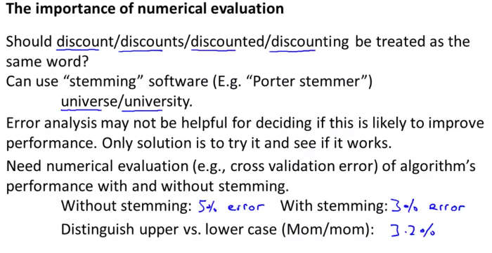
It is very important to get error results as a single, numerical value. Otherwise it is difficult to assess your algorithm's performance. For example if we use stemming, which is the process of treating the same word with different forms (fail/failing/failed) as one word (fail), and get a 3% error rate instead of 5%, then we should definitely add it to our model. However, if we try to distinguish between upper case and lower case letters and end up getting a 3.2% error rate instead of 3%, then we should avoid using this new feature. Hence, we should try new things, get a numerical value for our error rate, and based on our result decide whether we want to keep the new feature or not.
Video: Error Metrics for Skewed Classes
In the previous video, I talked about error analysis and the importance of having error metrics, that is of having a single real number evaluation metric for your learning algorithm to tell how well it's doing.
0:14
In the context of evaluation
0:16
and of error metrics, there is one important case, where it's particularly tricky to come up with an appropriate error metric, or evaluation metric, for your learning algorithm.
0:28
That case is the case of what's called skewed classes.
0:32
Let me tell you what that means.
0:36
Consider the problem of cancer classification, where we have features of medical patients and we want to decide whether or not they have cancer. So this is like the malignant versus benign tumor classification example that we had earlier.
0:51
So let's say y equals 1 if the patient has cancer and y equals 0 if they do not. We have trained the progression classifier and let's say we test our classifier on a test set and find that we get 1 percent error. So, we're making 99% correct diagnosis. Seems like a really impressive result, right. We're correct 99% percent of the time.
1:12
But now, let's say we find out that only 0.5 percent of patients in our training test sets actually have cancer. So only half a percent of the patients that come through our screening process have cancer.
1:26
In this case, the 1% error no longer looks so impressive.
1:31
And in particular, here's a piece of code, here's actually a piece of non learning code that takes this input of features x and it ignores it. It just sets y equals 0 and always predicts, you know, nobody has cancer and this algorithm would actually get 0.5 percent error. So this is even better than the 1% error that we were getting just now and this is a non learning algorithm that you know, it is just predicting y equals 0 all the time.
1:57
So this setting of when the ratio of positive to negative examples is very close to one of two extremes, where, in this case, the number of positive examples is much, much smaller than the number of negative examples because y equals one so rarely, this is what we call the case of skewed classes.
2:20
We just have a lot more of examples from one class than from the other class. And by just predicting y equals 0 all the time, or maybe our predicting y equals 1 all the time, an algorithm can do pretty well. So the problem with using classification error or classification accuracy as our evaluation metric is the following.
2:40
Let's say you have one joining algorithm that's getting 99.2% accuracy.
2:46
So, that's a 0.8% error. Let's say you make a change to your algorithm and you now are getting 99.5% accuracy.
2:59
That is 0.5% error.
3:04
So, is this an improvement to the algorithm or not? One of the nice things about having a single real number evaluation metric is this helps us to quickly decide if we just need a good change to the algorithm or not. By going from 99.2% accuracy to 99.5% accuracy.
3:21
You know, did we just do something useful or did we just replace our code with something that just predicts y equals zero more often? So, if you have very skewed classes it becomes much harder to use just classification accuracy, because you can get very high classification accuracies or very low errors, and it's not always clear if doing so is really improving the quality of your classifier because predicting y equals 0 all the time doesn't seem like a particularly good classifier.
3:53
But just predicting y equals 0 more often can bring your error down to, you know, maybe as low as 0.5%. When we're faced with such a skewed classes therefore we would want to come up with a different error metric or a different evaluation metric. One such evaluation metric are what's called precision recall.
4:15
Let me explain what that is.
4:17
Let's say we are evaluating a classifier on the test set. For the examples in the test set the actual
4:25
class of that example in the test set is going to be either one or zero, right, if there is a binary classification problem.
4:33
And what our learning algorithm will do is it will, you know, predict some value for the class and our learning algorithm will predict the value for each example in my test set and the predicted value will also be either one or zero.
4:50
So let me draw a two by two table as follows, depending on a full of these entries depending on what was the actual class and what was the predicted class. If we have an example where the actual class is one and the predicted class is one then that's called
5:07
an example that's a true positive, meaning our algorithm predicted that it's positive and in reality the example is positive. If our learning algorithm predicted that something is negative, class zero, and the actual class is also class zero then that's what's called a true negative. We predicted zero and it actually is zero.
5:27
To find the other two boxes, if our learning algorithm predicts that the class is one but the
5:34
actual class is zero, then that's called a false positive.
5:39
So that means our algorithm for the patient is cancelled out in reality if the patient does not.
5:44
And finally, the last box is a zero, one. That's called a false negative because our algorithm predicted zero, but the actual class was one.
5:57
And so, we have this little sort of two by two table based on what was the actual class and what was the predicted class.
6:07
So here's a different way of evaluating the performance of our algorithm. We're going to compute two numbers. The first is called precision - and what that says is,
6:17
of all the patients where we've predicted that they have cancer,
6:20
what fraction of them actually have cancer?
6:24
So let me write this down, the precision of a classifier is the number of true positives divided by
6:32
the number that we predicted
6:37
as positive, right?
6:39
So of all the patients that we went to those patients and we told them, "We think you have cancer." Of all those patients, what fraction of them actually have cancer? So that's called precision. And another way to write this would be true positives and then in the denominator is the number of predicted positives, and so that would be the sum of the, you know, entries in this first row of the table. So it would be true positives divided by true positives. I'm going to abbreviate positive as POS and then plus false positives, again abbreviating positive using POS.
7:20
So that's called precision, and as you can tell high precision would be good. That means that all the patients that we went to and we said, "You know, we're very sorry. We think you have cancer," high precision means that of that group of patients most of them we had actually made accurate predictions on them and they do have cancer.
7:38
The second number we're going to compute is called recall, and what recall say is, if all the patients in, let's say, in the test set or the cross-validation set, but if all the patients in the data set that actually have cancer,
7:52
what fraction of them that we correctly detect as having cancer. So if all the patients have cancer, how many of them did we actually go to them and you know, correctly told them that we think they need treatment.
8:05
So, writing this down, recall is defined as the number of positives, the number of true positives, meaning the number of people that have cancer and that we correctly predicted have cancer
8:20
and we take that and divide that by, divide that by the number of actual positives,
8:31
so this is the right number of actual positives of all the people that do have cancer. What fraction do we directly flag and you know, send the treatment.
8:40
So, to rewrite this in a different form, the denominator would be the number of actual positives as you know, is the sum of the entries in this first column over here.
8:50
And so writing things out differently, this is therefore, the number of true positives, divided by
8:59
the number of true positives
9:02
plus the number of
9:06
false negatives.
9:09
And so once again, having a high recall would be a good thing.
9:14
So by computing precision and recall this will usually give us a better sense of how well our classifier is doing.
9:21
And in particular if we have a learning algorithm that predicts y equals zero all the time, if it predicts no one has cancer, then this classifier will have a recall equal to zero, because there won't be any true positives and so that's a quick way for us to recognize that, you know, a classifier that predicts y equals 0 all the time, just isn't a very good classifier. And more generally, even for settings where we have very skewed classes, it's not possible for an algorithm to sort of "cheat" and somehow get a very high precision and a very high recall by doing some simple thing like predicting y equals 0 all the time or predicting y equals 1 all the time. And so we're much more sure that a classifier of a high precision or high recall actually is a good classifier, and this gives us a more useful evaluation metric that is a more direct way to actually understand whether, you know, our algorithm may be doing well.
10:21
So one final note in the definition of precision and recall, that we would define precision and recall, usually we use the convention that y is equal to 1, in the presence of the more rare class. So if we are trying to detect. rare conditions such as cancer, hopefully that's a rare condition, precision and recall are defined setting y equals 1, rather than y equals 0, to be sort of that the presence of that rare class that we're trying to detect. And by using precision and recall, we find, what happens is that even if we have very skewed classes, it's not possible for an algorithm to you know, "cheat" and predict y equals 1 all the time, or predict y equals 0 all the time, and get high precision and recall. And in particular, if a classifier is getting high precision and high recall, then we are actually confident that the algorithm has to be doing well, even if we have very skewed classes.
11:18
So for the problem of skewed classes precision recall gives us more direct insight into how the learning algorithm is doing and this is often a much better way to evaluate our learning algorithms, than looking at classification error or classification accuracy, when the classes are very skewed.
Video: Trading Off Precision and Recall
In the last video, we talked about precision and recall as an evaluation metric for classification problems with skewed constants. For many applications, we'll want to somehow control the trade-off between precision and recall. Let me tell you how to do that and also show you some even more effective ways to use precision and recall as an evaluation metric for learning algorithms.
0:28
As a reminder, here are the definitions of precision and recall from the previous video.
0:35
Let's continue our cancer classification example, where y equals 1 if the patient has cancer and y equals 0 otherwise. And let's say we're trained in logistic regression classifier which outputs probability between 0 and 1. So, as usual, we're going to predict 1, y equals 1, if h(x) is greater or equal to 0.5. And predict 0 if the hypothesis outputs a value less than 0.5. And this classifier may give us some value for precision and some value for recall.
1:10
But now, suppose we want to predict that the patient has cancer only if we're very confident that they really do. Because if you go to a patient and you tell them that they have cancer, it's going to give them a huge shock. What we give is a seriously bad news, and they may end up going through a pretty painful treatment process and so on. And so maybe we want to tell someone that we think they have cancer only if they are very confident. One way to do this would be to modify the algorithm, so that instead of setting this threshold at 0.5, we might instead say that we will predict that y is equal to 1 only if h(x) is greater or equal to 0.7. So this is like saying, we'll tell someone they have cancer only if we think there's a greater than or equal to, 70% chance that they have cancer.
2:00
And, if you do this, then you're predicting someone has cancer only when you're more confident and so you end up with a classifier that has higher precision. Because all of the patients that you're going to and saying, we think you have cancer, although those patients are now ones that you're pretty confident actually have cancer. And so a higher fraction of the patients that you predict have cancer will actually turn out to have cancer because making those predictions only if we're pretty confident.
2:34
But in contrast this classifier will have lower recall because now we're going to make predictions, we're going to predict y = 1 on a smaller number of patients. Now, can even take this further. Instead of setting the threshold at 0.7, we can set this at 0.9. Now we'll predict y=1 only if we are more than 90% certain that the patient has cancer. And so, a large fraction of those patients will turn out to have cancer. And so this would be a higher precision classifier will have lower recall because we want to correctly detect that those patients have cancer. Now consider a different example. Suppose we want to avoid missing too many actual cases of cancer, so we want to avoid false negatives. In particular, if a patient actually has cancer, but we fail to tell them that they have cancer then that can be really bad. Because if we tell a patient that they don't have cancer, then they're not going to go for treatment. And if it turns out that they have cancer, but we fail to tell them they have cancer, well, they may not get treated at all. And so that would be a really bad outcome because they die because we told them that they don't have cancer. They fail to get treated, but it turns out they actually have cancer. So, suppose that, when in doubt, we want to predict that y=1. So, when in doubt, we want to predict that they have cancer so that at least they look further into it, and these can get treated in case they do turn out to have cancer.
4:04
In this case, rather than setting higher probability threshold, we might instead take this value and instead set it to a lower value. So maybe 0.3 like so, right? And by doing so, we're saying that, you know what, if we think there's more than a 30% chance that they have cancer we better be more conservative and tell them that they may have cancer so that they can seek treatment if necessary.
4:31
And in this case what we would have is going to be a higher recall classifier, because we're going to be correctly flagging a higher fraction of all of the patients that actually do have cancer. But we're going to end up with lower precision because a higher fraction of the patients that we said have cancer, a high fraction of them will turn out not to have cancer after all.
5:00
And by the way, just as a sider, when I talk about this to other students, I've been told before, it's pretty amazing, some of my students say, is how I can tell the story both ways. Why we might want to have higher precision or higher recall and the story actually seems to work both ways. But I hope the details of the algorithm is true and the more general principle is depending on where you want, whether you want higher precision- lower recall, or higher recall- lower precision. You can end up predicting y=1 when h(x) is greater than some threshold. And so in general, for most classifiers there is going to be a trade off between precision and recall, and as you vary the value of this threshold that we join here, you can actually plot out some curve that trades off precision and recall. Where a value up here, this would correspond to a very high value of the threshold, maybe threshold equals 0.99. So that's saying, predict y=1 only if we're more than 99% confident, at least 99% probability this one. So that would be a high precision, relatively low recall. Where as the point down here, will correspond to a value of the threshold that's much lower, maybe equal 0.01, meaning, when in doubt at all, predict y=1, and if you do that, you end up with a much lower precision, higher recall classifier. And as you vary the threshold, if you want you can actually trace of a curve for your classifier to see the range of different values you can get for precision recall. And by the way, the precision-recall curve can look like many different shapes. Sometimes it will look like this, sometimes it will look like that. Now there are many different possible shapes for the precision-recall curve, depending on the details of the classifier. So, this raises another interesting question which is, is there a way to choose this threshold automatically? Or more generally, if we have a few different algorithms or a few different ideas for algorithms, how do we compare different precision recall numbers? Concretely, suppose we have three different learning algorithms. So actually, maybe these are three different learning algorithms, maybe these are the same algorithm but just with different values for the threshold. How do we decide which of these algorithms is best? One of the things we talked about earlier is the importance of a single real number evaluation metric. And that is the idea of having a number that just tells you how well is your classifier doing. But by switching to the precision recall metric we've actually lost that. We now have two real numbers. And so we often, we end up face the situations like if we trying to compare Algorithm 1 and Algorithm 2, we end up asking ourselves, is the precision of 0.5 and a recall of 0.4, was that better or worse than a precision of 0.7 and recall of 0.1? And, if every time you try out a new algorithm you end up having to sit around and think, well, maybe 0.5/0.4 is better than 0.7/0.1, or maybe not, I don't know. If you end up having to sit around and think and make these decisions, that really slows down your decision making process for what changes are useful to incorporate into your algorithm.
8:23
Whereas in contrast, if we have a single real number evaluation metric like a number that just tells us is algorithm 1 or is algorithm 2 better, then that helps us to much more quickly decide which algorithm to go with. It helps us as well to much more quickly evaluate different changes that we may be contemplating for an algorithm. So how can we get a single real number evaluation metric?
8:47
One natural thing that you might try is to look at the average precision and recall. So, using P and R to denote precision and recall, what you could do is just compute the average and look at what classifier has the highest average value.
9:00
But this turns out not to be such a good solution, because similar to the example we had earlier it turns out that if we have a classifier that predicts y=1 all the time, then if you do that you can get a very high recall, but you end up with a very low value of precision. Conversely, if you have a classifier that predicts y equals zero, almost all the time, that is that it predicts y=1 very sparingly, this corresponds to setting a very high threshold using the notation of the previous y. Then you can actually end up with a very high precision with a very low recall. So, the two extremes of either a very high threshold or a very low threshold, neither of that will give a particularly good classifier. And the way we recognize that is by seeing that we end up with a very low precision or a very low recall. And if you just take the average of (P+R)/2 from this example, the average is actually highest for Algorithm 3, even though you can get that sort of performance by predicting y=1 all the time and that's just not a very good classifier, right? You predict y=1 all the time, just normal useful classifier, but all it does is prints out y=1. And so Algorithm 1 or Algorithm 2 would be more useful than Algorithm 3. But in this example, Algorithm 3 has a higher average value of precision recall than Algorithms 1 and 2. So we usually think of this average of precision and recall as not a particularly good way to evaluate our learning algorithm.
10:38
In contrast, there's a different way for combining precision and recall. This is called the F Score and it uses that formula. And so in this example, here are the F Scores. And so we would tell from these F Scores, it looks like Algorithm 1 has the highest F Score, Algorithm 2 has the second highest, and Algorithm 3 has the lowest. And so, if we go by the F Score we would pick probably Algorithm 1 over the others.
11:04
The F Score, which is also called the F1 Score, is usually written F1 Score that I have here, but often people will just say F Score, either term is used. Is a little bit like taking the average of precision and recall, but it gives the lower value of precision and recall, whichever it is, it gives it a higher weight. And so, you see in the numerator here that the F Score takes a product of precision and recall. And so if either precision is 0 or recall is equal to 0, the F Score will be equal to 0. So in that sense, it kind of combines precision and recall, but for the F Score to be large, both precision and recall have to be pretty large. I should say that there are many different possible formulas for combing precision and recall. This F Score formula is really maybe a, just one out of a much larger number of possibilities, but historically or traditionally this is what people in Machine Learning seem to use. And the term F Score, it doesn't really mean anything, so don't worry about why it's called F Score or F1 Score.
12:09
But this usually gives you the effect that you want because if either a precision is zero or recall is zero, this gives you a very low F Score, and so to have a high F Score, you kind of need a precision or recall to be one. And concretely, if P=0 or R=0, then this gives you that the F Score = 0. Whereas a perfect F Score, so if precision equals one and recall equals 1, that will give you an F Score,
12:43
that's equal to 1 times 1 over 2 times 2, so the F Score will be equal to 1, if you have perfect precision and perfect recall. And intermediate values between 0 and 1, this usually gives a reasonable rank ordering of different classifiers.
13:00
So in this video, we talked about the notion of trading off between precision and recall, and how we can vary the threshold that we use to decide whether to predict y=1 or y=0. So it's the threshold that says, do we need to be at least 70% confident or 90% confident, or whatever before we predict y=1. And by varying the threshold, you can control a trade off between precision and recall. We also talked about the F Score, which takes precision and recall, and again, gives you a single real number evaluation metric. And of course, if your goal is to automatically set that threshold to decide what's really y=1 and y=0, one pretty reasonable way to do that would also be to try a range of different values of thresholds. So you try a range of values of thresholds and evaluate these different thresholds on, say, your cross-validation set and then to pick whatever value of threshold gives you the highest F Score on your crossvalidation [INAUDIBLE]. And that be a pretty reasonable way to automatically choose the threshold for your classifier as well.
Video: Data For Machine Learning
In the previous video, we talked about evaluation metrics.
0:04
In this video, I'd like to switch tracks a bit and touch on another important aspect of machine learning system design, which will often come up, which is the issue of how much data to train on. Now, in some earlier videos, I had cautioned against blindly going out and just spending lots of time collecting lots of data, because it's only sometimes that that would actually help.
0:27
But it turns out that under certain conditions, and I will say in this video what those conditions are, getting a lot of data and training on a certain type of learning algorithm, can be a very effective way to get a learning algorithm to do very good performance.
0:42
And this arises often enough that if those conditions hold true for your problem and if you're able to get a lot of data, this could be a very good way to get a very high performance learning algorithm.
0:53
So in this video, let's talk more about that. Let me start with a story.
1:01
Many, many years ago, two researchers that I know, Michelle Banko and Eric Broule ran the following fascinating study.
1:09
They were interested in studying the effect of using different learning algorithms versus trying them out on different training set sciences, they were considering the problem of classifying between confusable words, so for example, in the sentence: for breakfast I ate, should it be to, two or too? Well, for this example, for breakfast I ate two, 2 eggs.
1:33
So, this is one example of a set of confusable words and that's a different set. So they took machine learning problems like these, sort of supervised learning problems to try to categorize what is the appropriate word to go into a certain position in an English sentence.
1:51
They took a few different learning algorithms which were, you know, sort of considered state of the art back in the day, when they ran the study in 2001, so they took a variance, roughly a variance on logistic regression called the Perceptron. They also took some of their algorithms that were fairly out back then but somewhat less used now so when the algorithm also very similar to which is a regression but different in some ways, much used somewhat less, used not too much right now took what's called a memory based learning algorithm again used somewhat less now. But I'll talk a little bit about that later. And they used a naive based algorithm, which is something they'll actually talk about in this course. The exact algorithms of these details aren't important. Think of this as, you know, just picking four different classification algorithms and really the exact algorithms aren't important.
2:41
But what they did was they varied the training set size and tried out these learning algorithms on the range of training set sizes and that's the result they got. And the trends are very clear right first most of these outer rooms give remarkably similar performance. And second, as the training set size increases, on the horizontal axis is the training set size in millions
3:04
go from you know a hundred thousand up to a thousand million that is a billion training examples. The performance of the algorithms
3:12
all pretty much monotonically increase and the fact that if you pick any algorithm may be pick a "inferior algorithm" but if you give that "inferior algorithm" more data, then from these examples, it looks like it will most likely beat even a "superior algorithm".
3:32
So since this original study which is very influential, there's been a range of many different studies showing similar results that show that many different learning algorithms you know tend to, can sometimes, depending on details, can give pretty similar ranges of performance, but what can really drive performance is you can give the algorithm a ton of training data.
3:53
And this is, results like these has led to a saying in machine learning that often in machine learning it's not who has the best algorithm that wins, it's who has the
4:02
most data So when is this true and when is this not true? Because we have a learning algorithm for which this is true then getting a lot of data is often maybe the best way to ensure that we have an algorithm with very high performance rather than you know, debating worrying about exactly which of these items to use.
4:21
Let's try to lay out a set of assumptions under which having a massive training set we think will be able to help.
4:29
Let's assume that in our machine learning problem, the features x have sufficient information with which we can use to predict y accurately.
4:40
For example, if we take the confusable words all of them that we had on the previous slide. Let's say that it features x capture what are the surrounding words around the blank that we're trying to fill in. So the features capture then we want to have, sometimes for breakfast I have black eggs. Then yeah that is pretty much information to tell me that the word I want in the middle is TWO and that is not word TO and its not the word TOO. So
5:09
the features capture, you know, one of these surrounding words then that gives me enough information to pretty unambiguously decide what is the label y or in other words what is the word that I should be using to fill in that blank out of this set of three confusable words.
5:27
So that's an example what the future ex has sufficient information for specific y. For a counter example.
5:34
Consider a problem of predicting the price of a house from only the size of the house and from no other
5:42
features. So if you imagine I tell you that a house is, you know, 500 square feet but I don't give you any other features. I don't tell you that the house is in an expensive part of the city. Or if I don't tell you that the house, the number of rooms in the house, or how nicely furnished the house is, or whether the house is new or old. If I don't tell you anything other than that this is a 500 square foot house, well there's so many other factors that would affect the price of a house other than just the size of a house that if all you know is the size, it's actually very difficult to predict the price accurately.
6:16
So that would be a counter example to this assumption that the features have sufficient information to predict the price to the desired level of accuracy. The way I think about testing this assumption, one way I often think about it is, how often I ask myself.
6:30
Given the input features x, given the features, given the same information available as well as learning algorithm.
6:36
If we were to go to human expert in this domain. Can a human experts actually or can human expert confidently predict the value of y. For this first example if we go to, you know an expert human English speaker. You go to someone that speaks English well, right, then a human expert in English just read most people like you and me will probably we would probably be able to predict what word should go in here, to a good English speaker can predict this well, and so this gives me confidence that x allows us to predict y accurately, but in contrast if we go to an expert in human prices. Like maybe an expert realtor, right, someone who sells houses for a living. If I just tell them the size of a house and I tell them what the price is well even an expert in pricing or selling houses wouldn't be able to tell me and so this is fine that for the housing price example knowing only the size doesn't give me enough information to predict the price of the house. So, let's say, this assumption holds.
7:41
Let's see then, when having a lot of data could help. Suppose the features have enough information to predict the value of y. And let's suppose we use a learning algorithm with a large number of parameters so maybe logistic regression or linear regression with a large number of features. Or one thing that I sometimes do, one thing that I often do actually is using neural network with many hidden units. That would be another learning algorithm with a lot of parameters.
8:08
So these are all powerful learning algorithms with a lot of parameters that can fit very complex functions.
8:16
So, I'm going to call these, I'm
8:18
going to think of these as low-bias algorithms because you know we can fit very complex functions
8:25
and because we have a very powerful learning algorithm, they can fit very complex functions.
8:31
Chances are, if we run these algorithms on the data sets, it will be able to fit the training set well, and so hopefully the training error will be slow.
8:44
Now let's say, we use a massive, massive training set, in that case, if we have a huge training set, then hopefully even though we have a lot of parameters but if the training set is sort of even much larger than the number of parameters then hopefully these albums will be unlikely to overfit.
9:02
Right because we have such a massive training set and by unlikely to overfit what that means is that the training error will hopefully be close to the test error. Finally putting these two together that the train set error is small and the test set error is close to the training error what this two together imply is that hopefully the test set error
9:27
will also be small.
9:30
Another way to think about this is that in order to have a high performance learning algorithm we want it not to have high bias and not to have high variance.
9:42
So the bias problem we're going to address by making sure we have a learning algorithm with many parameters and so that gives us a low bias alorithm
9:50
and by using a very large training set, this ensures that we don't have a variance problem here. So hopefully our algorithm will have no variance and so is by pulling these two together, that we end up with a low bias and a low variance
10:04
learning algorithm and this allows us to do well on the test set. And fundamentally it's a key ingredients of assuming that the features have enough information and we have a rich class of functions that's why it guarantees low bias,
10:20
and then it having a massive training set that that's what guarantees more variance.
10:27
So this gives us a set of conditions rather hopefully some understanding of what's the sort of problem where if you have a lot of data and you train a learning algorithm with lot of parameters, that might be a good way to give a high performance learning algorithm and really, I think the key test that I often ask myself are first, can a human experts look at the features x and confidently predict the value of y. Because that's sort of a certification that y can be predicted accurately from the features x and second, can we actually get a large training set, and train the learning algorithm with a lot of parameters in the training set and if you can't do both then that's more often give you a very kind performance learning algorithm.
Reading: Lecture Slides
Support Vector Machines
Support vector machines, or SVMs, is a machine learning algorithm for classification. We introduce the idea and intuitions behind SVMs and discuss how to use it in practice.
6 videos, 1 reading
Video: Optimization Objective
By now, you've seen a range of difference learning algorithms. With supervised learning, the performance of many supervised learning algorithms will be pretty similar, and what matters less often will be whether you use learning algorithm a or learning algorithm b, but what matters more will often be things like the amount of data you create these algorithms on, as well as your skill in applying these algorithms. Things like your choice of the features you design to give to the learning algorithms, and how you choose the colorization parameter, and things like that. But, there's one more algorithm that is very powerful and is very widely used both within industry and academia, and that's called the support vector machine. And compared to both logistic regression and neural networks, the Support Vector Machine, or SVM sometimes gives a cleaner, and sometimes more powerful way of learning complex non-linear functions. And so let's take the next videos to talk about that. Later in this course, I will do a quick survey of a range of different supervisory algorithms just as a very briefly describe them. But the support vector machine, given its popularity and how powerful it is, this will be the last of the supervisory algorithms that I'll spend a significant amount of time on in this course as with our development other learning algorithms, we're gonna start by talking about the optimization objective. So, let's get started on this algorithm.
1:29
In order to describe the support vector machine, I'm actually going to start with logistic regression, and show how we can modify it a bit, and get what is essentially the support vector machine. So in logistic regression, we have our familiar form of the hypothesis there and the sigmoid activation function shown on the right.
1:50
And in order to explain some of the math, I'm going to use z to denote theta transpose axiom.
1:57
Now let's think about what we would like logistic regression to do. If we have an example with y equals one and by this I mean an example in either the training set or the test set or the cross-validation set, but when y is equal to one then we're sort of hoping that h of x will be close to one. Right, we're hoping to correctly classify that example. And what having x subscript 1, what that means is that theta transpose x must be must larger than 0. So there's greater than, greater than sign that means much, much greater than 0. And that's because it is z, the theta of transpose x is when z is much bigger than 0 is far to the right of the sphere. That the outputs of logistic progression becomes close to one.
2:44
Conversely, if we have an example where y is equal to zero, then what we're hoping for is that the hypothesis will output a value close to zero. And that corresponds to theta transpose x of z being much less than zero because that corresponds to a hypothesis of putting a value close to zero.
3:02
If you look at the cost function of logistic regression, what you'll find is that each example (x,y) contributes a term like this to the overall cost function, right?
3:14
So for the overall cost function, we will also have a sum over all the chain examples and the 1 over m term, that this expression here, that's the term that a single training example contributes to the overall objective function so we can just rush them.
3:32
Now if I take the definition for the fall of my hypothesis and plug it in over here, then what I get is that each training example contributes this term, ignoring the one over M but it contributes that term to my overall cost function for logistic regression.
3:51
Now let's consider two cases of when y is equal to one and when y is equal to zero. In the first case, let's suppose that y is equal to 1. In that case, only this first term in the objective matters, because this one minus y term would be equal to zero if y is equal to one.
4:13
So when y is equal to one, when in our example x comma y, when y is equal to 1 what we get is this term.. Minus log one over one, plus E to the negative Z where as similar to the last line I'm using Z to denote data transposed X and of course in a cost I should have this minus line that we just had if Y is equal to one so that's equal to one I just simplify in a way in the expression that I have written down here.
4:41
And if we plot this function as a function of z, what you find is that you get this curve shown on the lower left of the slide. And thus, we also see that when z is equal to large, that is, when theta transpose x is large, that corresponds to a value of z that gives us a fairly small value, a very, very small contribution to the consumption. And this kinda explains why, when logistic regression sees a positive example, with y=1, it tries to set theta transport x to be very large because that corresponds to this term, in the cross function, being small. Now, to fill the support vec machine, here's what we're going to do. We're gonna take this cross function, this minus log 1 over 1 plus e to negative z, and modify it a little bit. Let me take this point 1 over here, and let me draw the cross functions you're going to use. The new pass functions can be flat from here on out, and then we draw something that grows as a straight line, similar to logistic regression. But this is going to be a straight line at this portion. So the curve that I just drew in magenta, and the curve I just drew purple and magenta, so if it's pretty close approximation to the cross function used by logistic regression. Except it is now made up of two line segments, there's this flat portion on the right, and then there's this straight line portion on the left. And don't worry too much about the slope of the straight line portion. It doesn't matter that much. But that's the new cost function we're going to use for when y is equal to one, and you can imagine it should do something pretty similar to logistic regression. But turns out, that this will give the support vector machine computational advantages and give us, later on, an easier optimization problem
6:38
that would be easier for software to solve. We just talked about the case of y equals one. The other case is if y is equal to zero. In that case, if you look at the cost, then only the second term will apply because the first term goes away, right? If y is equal to zero, then you have a zero here, so you're left only with the second term of the expression above. And so the cost of an example, or the contribution of the cost function, is going to be given by this term over here. And if you plot that as a function of z, to have pure z on the horizontal axis, you end up with this one. And for the support vector machine, once again, we're going to replace this blue line with something similar and at the same time we replace it with a new cost, this flat out here, this 0 out here. And that then grows as a straight line, like so. So let me give these two functions names. This function on the left I'm going to call cost subscript 1 of z, and this function of the right I'm gonna call cost subscript 0 of z. And the subscript just refers to the cost corresponding to when y is equal to 1, versus when y Is equal to zero. Armed with these definitions, we're now ready to build a support vector machine. Here's the cost function, j of theta, that we have for logistic regression. In case this equation looks a bit unfamiliar, it's because previously we had a minus sign outside, but here what I did was I instead moved the minus signs inside these expressions, so it just makes it look a little different.
8:12
For the support vector machine what we're going to do is essentially take this and replace this with cost1 of z, that is cost1 of theta transpose x. And we're going to take this and replace it with cost0 of z, that is cost0 of theta transpose x. Where the cost one function is what we had on the previous slide that looks like this. And the cost zero function, again what we had on the previous slide, and it looks like this. So what we have for the support vector machine is a minimization problem of one over M, the sum of Y I times cost one, theta transpose X I, plus one minus Y I times cause zero of theta transpose X I, and then plus my usual regularization parameter.
9:21
Like so. Now, by convention, for the support of vector machine, we're actually write things slightly different. We re-parameterize this just very slightly differently.
9:33
First, we're going to get rid of the 1 over m terms, and this just this happens to be a slightly different convention that people use for support vector machines compared to or just a progression. But here's what I mean. You're one way to do this, we're just gonna get rid of these one over m terms and this should give you me the same optimal value of beta right? Because one over m is just as constant so whether I solved this minimization problem with one over n in front or not. I should end up with the same optimal value for theta. Here's what I mean, to give you an example, suppose I had a minimization problem. Minimize over a long number U of U minus five squared plus one. Well, the minimum of this happens to be U equals five.
10:23
Now if I were to take this objective function and multiply it by 10. So here my minimization problem is min over U, 10 U minus five squared plus 10. Well the value of U that minimizes this is still U equals five right? So multiply something that you're minimizing over, by some constant, 10 in this case, it does not change the value of U that gives us, that minimizes this function. So the same way, what I've done is by crossing out the M is all I'm doing is multiplying my objective function by some constant M and it doesn't change the value of theta. That achieves the minimum. The second bit of notational change, which is just, again, the more standard convention when using SVMs instead of logistic regression, is the following. So for logistic regression, we add two terms to the objective function. The first is this term, which is the cost that comes from the training set and the second is this row, which is the regularization term.
11:27
And what we had was we had a, we control the trade-off between these by saying, what we want is A plus, and then my regularization parameter lambda. And then times some other term B, where I guess I'm using your A to denote this first term, and I'm using B to denote the second term, maybe without the lambda.
11:51
And instead of prioritizing this as A plus lambda B, and so what we did was by setting different values for this regularization parameter lambda, we could trade off the relative weight between how much we wanted the training set well, that is, minimizing A, versus how much we care about keeping the values of the parameter small, so that will be, the parameter is B for the support vector machine, just by convention, we're going to use a different parameter. So instead of using lambda here to control the relative waiting between the first and second terms. We're instead going to use a different parameter which by convention is called C and is set to minimize C times a + B. So for logistic regression, if we set a very large value of lambda, that means you will give B a very high weight. Here is that if we set C to be a very small value, then that responds to giving B a much larger rate than C, than A. So this is just a different way of controlling the trade off, it's just a different way of prioritizing how much we care about optimizing the first term, versus how much we care about optimizing the second term. And if you want you can think of this as the parameter C playing a role similar to 1 over lambda. And it's not that it's two equations or these two expressions will be equal. This equals 1 over lambda, that's not the case. It's rather that if C is equal to 1 over lambda, then these two optimization objectives should give you the same value the same optimal value for theta so we just filling that in I'm gonna cross out lambda here and write in the constant C there.
13:37
So that gives us our overall optimization objective function for the support vector machine. And if you minimize that function, then what you have is the parameters learned by the SVM.
13:51
Finally unlike logistic regression, the support vector machine doesn't output the probability is that what we have is we have this cost function, that we minimize to get the parameter's data, and what a support vector machine does is it just makes a prediction of y being equal to one or zero, directly. So the hypothesis will predict one
14:13
if theta transpose x is greater or equal to zero, and it will predict zero otherwise and so having learned the parameters theta, this is the form of the hypothesis for the support vector machine. So that was a mathematical definition of what a support vector machine does. In the next few videos, let's try to get back to intuition about what this optimization objective leads to and whether the source of the hypotheses SVM will learn and we'll also talk about how to modify this just a little bit to the complex nonlinear functions.
Video: Large Margin Intuition
Sometimes people talk about support vector machines, as large margin classifiers, in this video I'd like to tell you what that means, and this will also give us a useful picture of what an SVM hypothesis may look like. Here's my cost function for the support vector machine
0:21
where here on the left I've plotted my cost 1 of z function that I used for positive examples and on the right I've plotted my
0:30
zero of 'Z' function, where I have 'Z' here on the horizontal axis. Now, let's think about what it takes to make these cost functions small.
0:39
If you have a positive example, so if y is equal to 1, then cost 1 of Z is zero only when Z is greater than or equal to 1. So in other words, if you have a positive example, we really want theta transpose x to be greater than or equal to 1 and conversely if y is equal to zero, look this cost zero of z function,
1:01
then it's only in this region where z is less than equal to 1 we have the cost is zero as z is equals to zero, and this is an interesting property of the support vector machine right, which is that, if you have a positive example so if y is equal to one, then all we really need is that theta transpose x is greater than equal to zero.
1:22
And that would mean that we classify correctly because if theta transpose x is greater than zero our hypothesis will predict zero. And similarly, if you have a negative example, then really all you want is that theta transpose x is less than zero and that will make sure we got the example right. But the support vector machine wants a bit more than that. It says, you know, don't just barely get the example right. So then don't just have it just a little bit bigger than zero. What i really want is for this to be quite a lot bigger than zero say maybe bit greater or equal to one and I want this to be much less than zero. Maybe I want it less than or equal to -1. And so this builds in an extra safety factor or safety margin factor into the support vector machine. Logistic regression does something similar too of course, but let's see what happens or let's see what the consequences of this are, in the context of the support vector machine.
2:14
Concretely, what I'd like to do next is consider a case case where we set this constant C to be a very large value, so let's imagine we set C to a very large value, may be a hundred thousand, some huge number.
2:29
Let's see what the support vector machine will do. If C is very, very large, then when minimizing
2:36
this optimization objective, we're going to be highly motivated to choose a value, so that this first term is equal to zero.
2:44
So let's try to understand the optimization problem in the context of, what would it take to make this first term in the objective equal to zero, because you know, maybe we'll set C to some huge constant, and this will hope, this should give us additional intuition about what sort of hypotheses a support vector machine learns. So we saw already that whenever you have a training example with a label of y=1 if you want to make that first term zero, what you need is is to find a value of theta so that theta transpose x i is greater than or equal to 1. And similarly, whenever we have an example, with label zero, in order to make sure that the cost, cost zero of Z, in order to make sure that cost is zero we need that theta transpose x i is less than or
3:37
equal to -1. So, if we think of our optimization problem as now, really choosing parameters and show that this first term is equal to zero, what we're left with is the following optimization problem. We're going to minimize that first term zero, so C times zero, because we're going to choose parameters so that's equal to zero, plus one half and then you know that second term and this first term is 'C' times zero, so let's just cross that out because I know that's going to be zero. And this will be subject to the constraint that theta transpose x(i) is greater than or equal to
4:18
one, if y(i)
4:22
Is equal to one and theta transpose x(i) is less than or equal to minus one whenever you have a negative example and it turns out that when you solve this optimization problem, when you minimize this as a function of the parameters theta
4:40
you get a very interesting decision boundary. Concretely, if you look at a data set like this with positive and negative examples, this data
4:50
is linearly separable and by that, I mean that there exists, you know, a straight line, altough there is many a different straight lines, they can separate the positive and negative examples perfectly. For example, here is one decision boundary
5:04
that separates the positive and negative examples, but somehow that doesn't look like a very natural one, right? Or by drawing an even worse one, you know here's another decision boundary that separates the positive and negative examples but just barely. But neither of those seem like particularly good choices.
5:20
The Support Vector Machines will instead choose this decision boundary, which I'm drawing in black.
5:29
And that seems like a much better decision boundary than either of the ones that I drew in magenta or in green. The black line seems like a more robust separator, it does a better job of separating the positive and negative examples. And mathematically, what that does is, this black decision boundary has a larger distance.
5:49
That distance is called the margin, when I draw up this two extra blue lines, we see that the black decision boundary has some larger minimum distance from any of my training examples, whereas the magenta and the green lines they come awfully close to the training examples.
6:04
and then that seems to do a less a good job separating the positive and negative classes than my black line. And so this distance is called the margin of the support vector machine and this gives the SVM a certain robustness, because it tries to separate the data with as a large a margin as possible.
6:29
So the support vector machine is sometimes also called a large margin classifier and this is actually a consequence of the optimization problem we wrote down on the previous slide. I know that you might be wondering how is it that the optimization problem I wrote down in the previous slide, how does that lead to this large margin classifier.
6:48
I know I haven't explained that yet. And in the next video I'm going to sketch a little bit of the intuition about why that optimization problem gives us this large margin classifier. But this is a useful feature to keep in mind if you are trying to understand what are the sorts of hypothesis that an SVM will choose. That is, trying to separate the positive and negative examples with as big a margin as possible.
7:12
I want to say one last thing about large margin classifiers in this intuition, so we wrote out this large margin classification setting in the case of when C, that regularization concept, was very large, I think I set that to a hundred thousand or something. So given a dataset like this, maybe we'll choose that decision boundary that separate the positive and negative examples on large margin.
7:37
Now, the SVM is actually sligthly more sophisticated than this large margin view might suggest. And in particular, if all you're doing is use a large margin classifier then your learning algorithms can be sensitive to outliers, so lets just add an extra positive example like that shown on the screen. If he had one example then it seems as if to separate data with a large margin,
8:02
maybe I'll end up learning a decision boundary like that, right? that is the magenta line and it's really not clear that based on the single outlier based on a single example and it's really not clear that it's actually a good idea to change my decision boundary from the black one over to the magenta one.
8:20
So, if C, if the regularization parameter C were very large, then this is actually what SVM will do, it will change the decision boundary from the black to the magenta one but if C were reasonably small if you were to use the C, not too large then you still end up with this black decision boundary. And of course if the data were not linearly separable so if you had some positive examples in here, or if you had some negative examples in here then the SVM will also do the right thing. And so this picture of a large margin classifier that's really, that's really the picture that gives better intuition only for the case of when the regulations parameter C is very large, and just to remind you this corresponds C plays a role similar to one over Lambda, where Lambda is the regularization parameter we had previously. And so it's only of one over Lambda is very large or equivalently if Lambda is very small that you end up with things like this Magenta decision boundary, but
9:28
in practice when applying support vector machines, when C is not very very large like that,
9:34
it can do a better job ignoring the few outliers like here. And also do fine and do reasonable things even if your data is not linearly separable. But when we talk about bias and variance in the context of support vector machines which will do a little bit later, hopefully all of of this trade-offs involving the regularization parameter will become clearer at that time. So I hope that gives some intuition about how this support vector machine functions as a large margin classifier that tries to separate the data with a large margin, technically this picture of this view is true only when the parameter C is very large, which is
10:10
a useful way to think about support vector machines.
10:13
There was one missing step in this video which is, why is it that the optimization problem we wrote down on these slides, how does that actually lead to the large margin classifier, I didn't do that in this video, in the next video I will sketch a little bit more of the math behind that to explain that separate reasoning of how the optimization problem we wrote out results in a large margin classifier.
Video: Mathematics Behind Large Margin Classification
In this video, I'd like to tell you a bit about the math behind large margin classification.
0:05
This video is optional, so please feel free to skip it. It may also give you better intuition about how the optimization problem of the support vex machine, how that leads to large margin classifiers.
0:21
In order to get started, let me first remind you of a couple of properties of what vector inner products look like.
0:28
Let's say I have two vectors U and V, that look like this. So both two dimensional vectors.
0:35
Then let's see what U transpose V looks like. And U transpose V is also called the inner products between the vectors U and V.
0:48
Use a two dimensional vector, so I can on plot it on this figure. So let's say that's the vector U. And what I mean by that is if on the horizontal axis that value takes whatever value U1 is and on the vertical axis the height of that is whatever U2 is the second component of the vector U. Now, one quantity that will be nice to have is the norm
1:16
of the vector U. So, these are, you know, double bars on the left and right that denotes the norm or length of U. So this just means; really the euclidean length of the vector U. And this is Pythagoras theorem is just equal to U1 squared plus U2 squared square root, right? And this is the length of the vector U. That's a real number. Just say you know, what is the length of this, what is the length of this vector down here. What is the length of this arrow that I just drew, is the normal view?
1:56
Now let's go back and look at the vector V because we want to compute the inner product. So V will be some other vector with, you know, some value V1, V2.
2:08
And so, the vector V will look like that, towards V like so.
2:16
Now let's go back and look at how to compute the inner product between U and V. Here's how you can do it. Let me take the vector V and project it down onto the vector U. So I'm going to take a orthogonal projection or a 90 degree projection, and project it down onto U like so.
2:36
And what I'm going to do measure length of this red line that I just drew here. So, I'm going to call the length of that red line P. So, P is the length or is the magnitude of the projection
2:49
of the vector V onto the vector U. Let me just write that down. So, P is the length
2:57
of the projection of the vector V onto the vector U. And it is possible to show that unit product U transpose V, that this is going to be equal to P times the norm or the length of the vector U. So, this is one way to compute the inner product. And if you actually do the geometry figure out what P is and figure out what the norm of U is. This should give you the same way, the same answer as the other way of computing unit product.
3:34
Right. Which is if you take U transpose V then U transposes this U1 U2, its a one by two matrix, 1 times V. And so this should actually give you U1, V1 plus U2, V2.
3:51
And so the theorem of linear algebra that these two formulas give you the same answer.
3:57
And by the way, U transpose V is also equal to V transpose U. So if you were to do the same process in reverse, instead of projecting V onto U, you could project U onto V. Then, you know, do the same process, but with the rows of U and V reversed. And you would actually, you should actually get the same number whatever that number is. And just to clarify what's going on in this equation the norm of U is a real number and P is also a real number. And so U transpose V is the regular multiplication as two real numbers of the length of P times the normal view.
4:35
Just one last detail, which is if you look at the norm of P, P is actually signed so to the right.
4:41
And it can either be positive or negative.
4:44
So let me say what I mean by that, if U is a vector that looks like this and V is a vector that looks like this.
4:52
So if the angle between U and V is greater than ninety degrees. Then if I project V onto U, what I get is a projection it looks like this and so that length P. And in this case, I will still have that U transpose V is equal to P times the norm of U. Except in this example P will be negative.
5:19
So, you know, in inner products if the angle between U and V is less than ninety degrees, then P is the positive length for that red line whereas if the angle of this angle of here is greater than 90 degrees then P here will be negative of the length of the super line of that little line segment right over there. So the inner product between two vectors can also be negative if the angle between them is greater than 90 degrees. So that's how vector inner products work. We're going to use these properties of vector inner product to try to understand the support vector machine optimization objective over there. Here is the optimization objective for the support vector machine that we worked out earlier. Just for the purpose of this slide I am going to make one simplification or once just to make the objective easy to analyze and what I'm going to do is ignore the indeceptrums. So, we'll just ignore theta 0 and set that to be equal to 0. To
6:16
make things easier to plot, I'm also going to set N the number of features to be equal to 2. So, we have only 2 features,
6:23
X1 and X2.
6:26
Now, let's look at the objective function. The optimization objective of the SVM. What we have only two features. When N is equal to 2. This can be written, one half of theta one squared plus theta two squared. Because we only have two parameters, theta one and thetaa two.
6:45
What I'm going to do is rewrite this a bit. I'm going to write this as one half of theta one squared plus theta two squared and the square root squared. And the reason I can do that, is because for any number, you know, W, right, the
7:00
square roots of W and then squared, that's just equal to W. So square roots and squared should give you the same thing.
7:08
What you may notice is that this term inside is that's equal to the norm
7:14
or the length of the vector theta and what I mean by that is that if we write out the vector theta like this, as you know theta one, theta two. Then this term that I've just underlined in red, that's exactly the length, or the norm, of the vector theta. We are calling the definition of the norm of the vector that we have on the previous line.
7:36
And in fact this is actually equal to the length of the vector theta, whether you write it as theta zero, theta 1, theta 2. That is, if theta zero is equal to zero, as I assume here. Or just the length of theta 1, theta 2; but for this line I am going to ignore theta 0. So let me just, you know, treat theta as this, let me just write theta, the normal theta as this theta 1, theta 2 only, but the math works out either way, whether we include theta zero here or not. So it's not going to matter for the rest of our derivation.
8:07
And so finally this means that my optimization objective is equal to one half of the norm of theta squared.
8:16
So all the support vector machine is doing in the optimization objective is it's minimizing the squared norm of the square length of the parameter vector theta.
8:28
Now what I'd like to do is look at these terms, theta transpose X and understand better what they're doing. So given the parameter vector theta and given and example x, what is this is equal to? And on the previous slide, we figured out what U transpose V looks like, with different vectors U and V. And so we're going to take those definitions, you know, with theta and X(i) playing the roles of U and V.
8:54
And let's see what that picture looks like. So, let's say I plot. Let's say I look at just a single training example. Let's say I have a positive example the drawing was across there and let's say that is my example X(i), what that really means is
9:12
plotted on the horizontal axis some value X(i) 1 and on the vertical axis
9:21
X(i) 2. That's how I plot my training examples.
9:25
And although we haven't been really thinking of this as a vector, what this really is, this is a vector from the origin from 0, 0 out to
9:34
the location of this training example.
9:37
And now let's say we have a parameter vector and I'm going to plot that as vector, as well. What I mean by that is if I plot theta 1 here and theta 2 there
9:56
so what is the inner product theta transpose X(i). While using our earlier method, the way we compute that is we take my example and project it onto my parameter vector theta.
10:09
And then I'm going to look at the length of this segment that I'm coloring in, in red. And I'm going to call that P superscript I to denote that this is a projection of the i-th training example
10:24
onto the parameter vector theta.
10:26
And so what we have is that theta transpose X(i) is equal to following what we have on the previous slide, this is going to be equal to
10:36
P times the length of the norm of the vector theta.
10:43
And this is of course also equal to theta 1 x1
10:47
plus theta 2 x2. So each of these is, you know, an equally valid way of computing the inner product between theta and X(i).
10:57
Okay. So where does this leave us? What this means is that, this constrains that theta transpose X(i) be greater than or equal to one or less than minus one. What this means is that it can replace the use of constraints that P(i) times X be greater than or equal to one. Because theta transpose X(i) is equal to P(i) times the norm of theta.
11:21
So writing that into our optimization objective. This is what we get where I have, instead of theta transpose X(i), I now have this P(i) times the norm of theta.
11:31
And just to remind you we worked out earlier too that this optimization objective can be written as one half times the norm of theta squared.
11:41
So, now let's consider the training example that we have at the bottom and for now, continuing to use the simplification that theta 0 is equal to 0. Let's see what decision boundary the support vector machine will choose.
11:55
Here's one option, let's say the support vector machine were to choose this decision boundary. This is not a very good choice because it has very small margins. This decision boundary comes very close to the training examples.
12:09
Let's see why the support vector machine will not do this.
12:14
For this choice of parameters it's possible to show that the parameter vector theta is actually at 90 degrees to the decision boundary. And so, that green decision boundary corresponds to a parameter vector theta that points in that direction.
12:30
And by the way, the simplification that theta 0 equals 0 that just means that the decision boundary must pass through the origin, (0,0) over there. So now, let's look at what this implies for the optimization objective.
12:45
Let's say that this example here.
12:47
Let's say that's my first example, you know,
12:50
X1.
12:51
If we look at the projection of this example onto my parameters theta.
12:56
That's the projection.
12:57
And so that little red line segment.
13:00
That is equal to P1. And that is going to be pretty small, right.
13:05
And similarly, if this
13:09
example here, if this happens to be X2, that's my second example.
13:13
Then, if I look at the projection of this this example onto theta.
13:18
You know. Then, let me draw this one in magenta.
13:21
This little magenta line segment, that's going to be P2. That's the projection of the second example onto my, onto the direction
13:30
of my parameter vector theta which goes like this.
13:33
And so, this little
13:35
projection line segment is getting pretty small.
13:36
P2 will actually be a negative number, right so P2 is in the opposite direction.
13:43
This vector has greater than 90 degree angle with my parameter vector theta, it's going to be less than 0.
13:50
And so what we're finding is that these terms P(i) are going to be pretty small numbers. So if we look at the optimization objective and see, well, for positive examples we need P(i) times the norm of theta to be bigger than either one.
14:08
But if P(i) over here, if P1 over here is pretty small, that means that we need the norm of theta to be pretty large, right? If
14:19
P1 of theta is small and we want P1 you know times in all of theta to be bigger than either one, well the only way for that to be true for the profit that these two numbers to be large if P1 is small, as we said we want the norm of theta to be large.
14:34
And similarly for our negative example, we need P2
14:39
times the norm of theta to be less than or equal to minus one. And we saw in this example already that P2 is going pretty small negative number, and so the only way for that to happen as well is for the norm of theta to be large, but what we are doing in the optimization objective is we are trying to find a setting of parameters where the norm of theta is small, and so you know, so this doesn't seem like such a good direction for the parameter vector and theta. In contrast, just look at a different decision boundary.
15:17
Here, let's say, this SVM chooses
15:20
that decision boundary.
15:22
Now the is going to be very different. If that is the decision boundary, here is the corresponding direction for theta. So, with the direction boundary you know, that vertical line that corresponds to it is possible to show using linear algebra that the way to get that green decision boundary is have the vector of theta be at 90 degrees to it, and now if you look at the projection of your data onto the vector
15:48
x, lets say its before this example is my example of x1. So when I project this on to x, or onto theta, what I find is that this is P1.
16:00
That length there is P1.
16:03
The other example, that example is and I do the same projection and what I find is that this length here is a P2 really that is going to be less than 0. And you notice that now P1 and P2, these lengths
16:23
of the projections are going to be much bigger, and so if we still need to enforce these constraints that P1 of the norm of theta is phase number one because P1 is so much bigger now. The normal can be smaller.
16:41
And so, what this means is that by choosing the decision boundary shown on the right instead of on the left, the SVM can make the norm of the parameters theta much smaller. So, if we can make the norm of theta smaller and therefore make the squared norm of theta smaller, which is why the SVM would choose this hypothesis on the right instead.
17:02
And this is how
17:05
the SVM gives rise to this large margin certification effect.
17:10
Mainly, if you look at this green line, if you look at this green hypothesis we want the projections of my positive and negative examples onto theta to be large, and the only way for that to hold true this is if surrounding the green line.
17:24
There's this large margin, there's this large gap that separates
17:33
positive and negative examples is really the magnitude of this gap. The magnitude of this margin is exactly the values of P1, P2, P3 and so on. And so by making the margin large, by these tyros P1, P2, P3 and so on that's the SVM can end up with a smaller value for the norm of theta which is what it is trying to do in the objective. And this is why this machine ends up with enlarge margin classifiers because itss trying to maximize the norm of these P1 which is the distance from the training examples to the decision boundary.
18:14
Finally, we did this whole derivation using this simplification that the parameter theta 0 must be equal to 0. The effect of that as I mentioned briefly, is that if theta 0 is equal to 0 what that means is that we are entertaining decision boundaries that pass through the origins of decision boundaries pass through the origin like that, if you allow theta zero to be non 0 then what that means is that you entertain the decision boundaries that did not cross through the origin, like that one I just drew. And I'm not going to do the full derivation that. It turns out that this same large margin proof works in pretty much in exactly the same way. And there's a generalization of this argument that we just went through them long ago through that shows that even when theta 0 is non 0, what the SVM is trying to do when you have this optimization objective.
19:08
Which again corresponds to the case of when C is very large.
19:14
But it is possible to show that, you know, when theta is not equal to 0 this support vector machine is still finding is really trying to find the large margin separator that between the positive and negative examples. So that explains how this support vector machine is a large margin classifier.
19:32
In the next video we will start to talk about how to take some of these SVM ideas and start to apply them to build a complex nonlinear classifiers.
Video: Kernels I
In this video, I'd like to start adapting support vector machines in order to develop complex nonlinear classifiers.
0:07
The main technique for doing that is something called kernels.
0:11
Let's see what this kernels are and how to use them.
0:15
If you have a training set that looks like this, and you want to find a nonlinear decision boundary to distinguish the positive and negative examples, maybe a decision boundary that looks like that.
0:27
One way to do so is to come up with a set of complex polynomial features, right? So, set of features that looks like this, so that you end up with a hypothesis X that predicts 1 if you know that theta 0 and plus theta 1 X1 plus dot dot dot all those polynomial features is greater than 0, and predict 0, otherwise.
0:51
And another way of writing this, to introduce a level of new notation that I'll use later, is that we can think of a hypothesis as computing a decision boundary using this. So, theta 0 plus theta 1 f1 plus theta 2, f2 plus theta 3, f3 plus and so on. Where I'm going to use this new denotation f1, f2, f3 and so on to denote these new sort of features
1:19
that I'm computing, so f1 is just X1, f2 is equal to X2, f3 is equal to this one here. So, X1X2. So, f4 is equal to
1:33
X1 squared where f5 is to be x2 squared and so on and we seen previously that coming up with these high order polynomials is one way to come up with lots more features,
1:45
the question is, is there a different choice of features or is there better sort of features than this high order polynomials because you know it's not clear that this high order polynomial is what we want, and what we talked about computer vision talk about when the input is an image with lots of pixels. We also saw how using high order polynomials becomes very computationally expensive because there are a lot of these higher order polynomial terms.
2:11
So, is there a different or a better choice of the features that we can use to plug into this sort of hypothesis form. So, here is one idea for how to define new features f1, f2, f3.
2:24
On this line I am going to define only three new features, but for real problems we can get to define a much larger number. But here's what I'm going to do in this phase of features X1, X2, and I'm going to leave X0 out of this, the interceptor X0, but in this phase X1 X2, I'm going to just,
2:42
you know, manually pick a few points, and then call these points l1, we are going to pick a different point, let's call that l2 and let's pick the third one and call this one l3, and for now let's just say that I'm going to choose these three points manually. I'm going to call these three points line ups, so line up one, two, three. What I'm going to do is define my new features as follows, given an example X, let me define my first feature f1 to be some measure of the similarity between my training example X and my first landmark and this specific formula that I'm going to use to measure similarity is going to be this is E to the minus the length of X minus l1, squared, divided by two sigma squared.
3:40
So, depending on whether or not you watched the previous optional video, this notation, you know, this is the length of the vector W. And so, this thing here, this X minus l1, this is actually just the euclidean distance
3:58
squared, is the euclidean distance between the point x and the landmark l1. We will see more about this later.
4:06
But that's my first feature, and my second feature f2 is going to be, you know, similarity function that measures how similar X is to l2 and the game is going to be defined as the following function.
4:25
This is E to the minus of the square of the euclidean distance between X and the second landmark, that is what the enumerator is and then divided by 2 sigma squared and similarly f3 is, you know, similarity between X and l3, which is equal to, again, similar formula.
4:46
And what this similarity function is, the mathematical term for this, is that this is going to be a kernel function. And the specific kernel I'm using here, this is actually called a Gaussian kernel.
5:00
And so this formula, this particular choice of similarity function is called a Gaussian kernel. But the way the terminology goes is that, you know, in the abstract these different similarity functions are called kernels and we can have different similarity functions
5:13
and the specific example I'm giving here is called the Gaussian kernel. We'll see other examples of other kernels. But for now just think of these as similarity functions.
5:22
And so, instead of writing similarity between X and l, sometimes we also write this a kernel denoted you know, lower case k between x and one of my landmarks all right.
5:34
So let's see what a criminals actually do and why these sorts of similarity functions, why these expressions might make sense.
5:46
So let's take my first landmark. My landmark l1, which is one of those points I chose on my figure just now.
5:53
So the similarity of the kernel between x and l1 is given by this expression.
5:57
Just to make sure, you know, we are on the same page about what the numerator term is, the numerator can also be written as a sum from J equals 1 through N on sort of the distance. So this is the component wise distance between the vector X and the vector l. And again for the purpose of these slides I'm ignoring X0. So just ignoring the intercept term X0, which is always equal to 1.
6:21
So, you know, this is how you compute the kernel with similarity between X and a landmark.
6:27
So let's see what this function does. Suppose X is close to one of the landmarks.
6:33
Then this euclidean distance formula and the numerator will be close to 0, right. So, that is this term here, the distance was great, the distance using X and 0 will be close to zero, and so
6:46
f1, this is a simple feature, will be approximately E to the minus 0 and then the numerator squared over 2 is equal to squared
6:55
so that E to the 0, E to minus 0, E to 0 is going to be close to one.
7:01
And I'll put the approximation symbol here because the distance may not be exactly 0, but if X is closer to landmark this term will be close to 0 and so f1 would be close 1.
7:13
Conversely, if X is far from 01 then this first feature f1 will be E to the minus of some large number squared, divided divided by two sigma squared and E to the minus of a large number is going to be close to 0.
7:33
So what these features do is they measure how similar X is from one of your landmarks and the feature f is going to be close to one when X is close to your landmark and is going to be 0 or close to zero when X is far from your landmark. Each of these landmarks. On the previous line, I drew three landmarks, l1, l2,l3.
7:56
Each of these landmarks, defines a new feature f1, f2 and f3. That is, given the the training example X, we can now compute three new features: f1, f2, and f3, given, you know, the three landmarks that I wrote just now. But first, let's look at this exponentiation function, let's look at this similarity function and plot in some figures and just, you know, understand better what this really looks like.
8:23
For this example, let's say I have two features X1 and X2. And let's say my first landmark, l1 is at a location, 3 5. So
8:33
and let's say I set sigma squared equals one for now. If I plot what this feature looks like, what I get is this figure. So the vertical axis, the height of the surface is the value
8:45
of f1 and down here on the horizontal axis are, if I have some training example, and there
8:51
is x1 and there is x2. Given a certain training example, the training example here which shows the value of x1 and x2 at a height above the surface, shows the corresponding value of f1 and down below this is the same figure I had showed, using a quantifiable plot, with x1 on horizontal axis, x2 on horizontal axis and so, this figure on the bottom is just a contour plot of the 3D surface.
9:16
You notice that when X is equal to 3 5 exactly, then we the f1 takes on the value 1, because that's at the maximum and X moves away as X goes further away then this feature takes on values
9:36
that are close to 0.
9:38
And so, this is really a feature, f1 measures, you know, how close X is to the first landmark and if varies between 0 and one depending on how close X is to the first landmark l1.
9:52
Now the other was due on this slide is show the effects of varying this parameter sigma squared. So, sigma squared is the parameter of the Gaussian kernel and as you vary it, you get slightly different effects.
10:05
Let's set sigma squared to be equal to 0.5 and see what we get. We set sigma square to 0.5, what you find is that the kernel looks similar, except for the width of the bump becomes narrower. The contours shrink a bit too. So if sigma squared equals to 0.5 then as you start from X equals 3 5 and as you move away,
10:24
then the feature f1 falls to zero much more rapidly and conversely,
10:32
if you has increase since where three in that case and as I move away from, you know l. So this point here is really l, right, that's l1 is at location 3 5, right. So it's shown up here.
10:48
And if sigma squared is large, then as you move away from l1, the value of the feature falls away much more slowly.
11:03
So, given this definition of the features, let's see what source of hypothesis we can learn.
11:09
Given the training example X, we are going to compute these features
11:14
f1, f2, f3 and a
11:17
hypothesis is going to predict one when theta 0 plus theta 1 f1 plus theta 2 f2, and so on is greater than or equal to 0. For this particular example, let's say that I've already found a learning algorithm and let's say that, you know, somehow I ended up with these values of the parameter. So if theta 0 equals minus 0.5, theta 1 equals 1, theta 2 equals 1, and theta 3 equals 0 And what I want to do is consider what happens if we have a training example that takes
11:49
has location at this magenta dot, right where I just drew this dot over here. So let's say I have a training example X, what would my hypothesis predict? Well, If I look at this formula.
12:04
Because my training example X is close to l1, we have that f1 is going to be close to 1 the because my training example X is far from l2 and l3 I have that, you know, f2 would be close to 0 and f3 will be close to 0.
12:21
So, if I look at that formula, I have theta 0 plus theta 1 times 1 plus theta 2 times some value. Not exactly 0, but let's say close to 0. Then plus theta 3 times something close to 0.
12:37
And this is going to be equal to plugging in these values now.
12:41
So, that gives minus 0.5 plus 1 times 1 which is 1, and so on. Which is equal to 0.5 which is greater than or equal to 0. So, at this point, we're going to predict Y equals 1, because that's greater than or equal to zero.
12:58
Now let's take a different point. Now lets' say I take a different point, I'm going to draw this one in a different color, in cyan say, for a point out there, if that were my training example X, then if you make a similar computation, you find that f1, f2,
13:15
Ff3 are all going to be close to 0.
13:18
And so, we have theta 0 plus theta 1, f1, plus so on and this will be about equal to minus 0.5, because theta 0 is minus 0.5 and f1, f2, f3 are all zero. So this will be minus 0.5, this is less than zero. And so, at this point out there, we're going to predict Y equals zero.
13:44
And if you do this yourself for a range of different points, be sure to convince yourself that if you have a training example that's close to L2, say, then at this point we'll also predict Y equals one.
13:56
And in fact, what you end up doing is, you know, if you look around this boundary, this space, what we'll find is that for points near l1 and l2 we end up predicting positive. And for points far away from l1 and l2, that's for points far away from these two landmarks, we end up predicting that the class is equal to 0. As so, what we end up doing,is that the decision boundary of this hypothesis would end up looking something like this where inside this red decision boundary would predict Y equals 1 and outside we predict
14:32
Y equals 0. And so this is how with this definition of the landmarks and of the kernel function. We can learn pretty complex non-linear decision boundary, like what I just drew where we predict positive when we're close to either one of the two landmarks. And we predict negative when we're very far away from any of the landmarks. And so this is part of the idea of kernels of and how we use them with the support vector machine, which is that we define these extra features using landmarks and similarity functions to learn more complex nonlinear classifiers.
15:08
So hopefully that gives you a sense of the idea of kernels and how we could use it to define new features for the Support Vector Machine.
15:15
But there are a couple of questions that we haven't answered yet. One is, how do we get these landmarks? How do we choose these landmarks? And another is, what other similarity functions, if any, can we use other than the one we talked about, which is called the Gaussian kernel. In the next video we give answers to these questions and put everything together to show how support vector machines with kernels can be a powerful way to learn complex nonlinear functions.
Video: Kernels II
In the last video, we started to talk about the kernels idea and how it can be used to define new features for the support vector machine. In this video, I'd like to throw in some of the missing details and, also, say a few words about how to use these ideas in practice. Such as, how they pertain to, for example, the bias variance trade-off in support vector machines.
0:22
In the last video, I talked about the process of picking a few landmarks. You know, l1, l2, l3 and that allowed us to define the similarity function also called the kernel or in this example if you have this similarity function this is a Gaussian kernel.
0:38
And that allowed us to build this form of a hypothesis function.
0:43
But where do we get these landmarks from? Where do we get l1, l2, l3 from? And it seems, also, that for complex learning problems, maybe we want a lot more landmarks than just three of them that we might choose by hand.
0:55
So in practice this is how the landmarks are chosen which is that given the machine learning problem. We have some data set of some some positive and negative examples. So, this is the idea here which is that we're gonna take the examples and for every training example that we have, we are just going to call it. We're just going to put landmarks as exactly the same locations as the training examples.
1:18
So if I have one training example if that is x1, well then I'm going to choose this is my first landmark to be at xactly the same location as my first training example.
1:29
And if I have a different training example x2. Well we're going to set the second landmark
1:35
to be the location of my second training example.
1:38
On the figure on the right, I used red and blue dots just as illustration, the color of this figure, the color of the dots on the figure on the right is not significant.
1:47
But what I'm going to end up with using this method is I'm going to end up with m landmarks of l1, l2
1:54
down to l(m) if I have m training examples with one landmark per location of my per location of each of my training examples. And this is nice because it is saying that my features are basically going to measure how close an example is to one of the things I saw in my training set. So, just to write this outline a little more concretely, given m training examples, I'm going to choose the the location of my landmarks to be exactly near the locations of my m training examples.
2:25
When you are given example x, and in this example x can be something in the training set, it can be something in the cross validation set, or it can be something in the test set. Given an example x we are going to compute, you know, these features as so f1, f2, and so on. Where l1 is actually equal to x1 and so on. And these then give me a feature vector. So let me write f as the feature vector. I'm going to take these f1, f2 and so on, and just group them into feature vector.
2:56
Take those down to fm.
2:59
And, you know, just by convention. If we want, we can add an extra feature f0, which is always equal to 1. So this plays a role similar to what we had previously. For x0, which was our interceptor.
3:13
So, for example, if we have a training example x(i), y(i),
3:18
the features we would compute for this training example will be as follows: given x(i), we will then map it to, you know, f1(i).
3:27
Which is the similarity. I'm going to abbreviate as SIM instead of writing out the whole word
3:35
similarity, right?
3:37
And f2(i) equals the similarity between x(i) and l2, and so on, down to fm(i) equals
3:49
the similarity between x(i) and l(m).
3:55
And somewhere in the middle. Somewhere in this list, you know, at the i-th component, I will actually have one feature component which is f subscript i(i), which is going to be the similarity
4:13
between x and l(i).
4:15
Where l(i) is equal to x(i), and so you know fi(i) is just going to be the similarity between x and itself.
4:23
And if you're using the Gaussian kernel this is actually e to the minus 0 over 2 sigma squared and so, this will be equal to 1 and that's okay. So one of my features for this training example is going to be equal to 1.
4:34
And then similar to what I have above. I can take all of these m features and group them into a feature vector. So instead of representing my example, using, you know, x(i) which is this what R(n) plus R(n) one dimensional vector.
4:48
Depending on whether you can set terms, is either R(n) or R(n) plus 1. We can now instead represent my training example using this feature vector f. I am going to write this f superscript i. Which is going to be taking all of these things and stacking them into a vector. So, f1(i) down to fm(i) and if you want and well, usually we'll also add this f0(i), where f0(i) is equal to 1. And so this vector here gives me my new feature vector with which to represent my training example. So given these kernels and similarity functions, here's how we use a simple vector machine. If you already have a learning set of parameters theta, then if you given a value of x and you want to make a prediction.
5:41
What we do is we compute the features f, which is now an R(m) plus 1 dimensional feature vector.
5:49
And we have m here because we have m training examples and thus m landmarks and what we do is we predict 1 if theta transpose f is greater than or equal to 0. Right. So, if theta transpose f, of course, that's just equal to theta 0, f0 plus theta 1, f1 plus dot dot dot, plus theta m f(m). And so my parameter vector theta is also now going to be an m plus 1 dimensional vector. And we have m here because where the number of landmarks is equal to the training set size. So m was the training set size and now, the parameter vector theta is going to be m plus one dimensional.
6:32
So that's how you make a prediction if you already have a setting for the parameter's theta. How do you get the parameter's theta? Well you do that using the SVM learning algorithm, and specifically what you do is you would solve this minimization problem. You've minimized the parameter's theta of C times this cost function which we had before. Only now, instead of looking there instead of making predictions using theta transpose x(i) using our original features, x(i). Instead we've taken the features x(i) and replace them with a new features
7:07
so we are using theta transpose f(i) to make a prediction on the i'f training examples and we see that, you know, in both places here and it's by solving this minimization problem that you get the parameters for your Support Vector Machine.
7:23
And one last detail is because this optimization problem we really have n equals m features. That is here. The number of features we have.
7:37
Really, the effective number of features we have is dimension of f. So that n is actually going to be equal to m. So, if you want to, you can think of this as a sum, this really is a sum from j equals 1 through m. And then one way to think about this, is you can think of it as n being equal to m, because if f isn't a new feature, then we have m plus 1 features, with the plus 1 coming from the interceptor.
8:05
And here, we still do sum from j equal 1 through n, because similar to our earlier videos on regularization, we still do not regularize the parameter theta zero, which is why this is a sum for j equals 1 through m instead of j equals zero though m. So that's the support vector machine learning algorithm. That's one sort of, mathematical detail aside that I should mention, which is that in the way the support vector machine is implemented, this last term is actually done a little bit differently. So you don't really need to know about this last detail in order to use support vector machines, and in fact the equations that are written down here should give you all the intuitions that should need. But in the way the support vector machine is implemented, you know, that term, the sum of j of theta j squared right?
8:53
Another way to write this is this can be written as theta transpose theta if we ignore the parameter theta 0. So theta 1 down to theta m. Ignoring theta 0.
9:11
Then this sum of j of theta j squared that this can also be written theta transpose theta.
9:19
And what most support vector machine implementations do is actually replace this theta transpose theta, will instead, theta transpose times some matrix inside, that depends on the kernel you use, times theta. And so this gives us a slightly different distance metric. We'll use a slightly different measure instead of minimizing exactly
9:41
the norm of theta squared means that minimize something slightly similar to it. That's like a rescale version of the parameter vector theta that depends on the kernel. But this is kind of a mathematical detail. That allows the support vector machine software to run much more efficiently.
9:58
And the reason the support vector machine does this is with this modification. It allows it to scale to much bigger training sets. Because for example, if you have a training set with 10,000 training examples.
10:12
Then, you know, the way we define landmarks, we end up with 10,000 landmarks.
10:16
And so theta becomes 10,000 dimensional. And maybe that works, but when m becomes really, really big then solving for all of these parameters, you know, if m were 50,000 or a 100,000 then solving for all of these parameters can become expensive for the support vector machine optimization software, thus solving the minimization problem that I drew here. So kind of as mathematical detail, which again you really don't need to know about.
10:41
It actually modifies that last term a little bit to optimize something slightly different than just minimizing the norm squared of theta squared, of theta. But if you want, you can feel free to think of this as an kind of a n implementational detail that does change the objective a bit, but is done primarily for reasons of computational efficiency, so usually you don't really have to worry about this.
11:07
And by the way, in case your wondering why we don't apply the kernel's idea to other algorithms as well like logistic regression, it turns out that if you want, you can actually apply the kernel's idea and define the source of features using landmarks and so on for logistic regression. But the computational tricks that apply for support vector machines don't generalize well to other algorithms like logistic regression. And so, using kernels with logistic regression is going too very slow, whereas, because of computational tricks, like that embodied and how it modifies this and the details of how the support vector machine software is implemented, support vector machines and kernels tend go particularly well together. Whereas, logistic regression and kernels, you know, you can do it, but this would run very slowly. And it won't be able to take advantage of advanced optimization techniques that people have figured out for the particular case of running a support vector machine with a kernel. But all this pertains only to how you actually implement software to minimize the cost function. I will say more about that in the next video, but you really don't need to know about how to write software to minimize this cost function because you can find very good off the shelf software for doing so.
12:18
And just as, you know, I wouldn't recommend writing code to invert a matrix or to compute a square root, I actually do not recommend writing software to minimize this cost function yourself, but instead to use off the shelf software packages that people have developed and so those software packages already embody these numerical optimization tricks,
12:39
so you don't really have to worry about them. But one other thing that is worth knowing about is when you're applying a support vector machine, how do you choose the parameters of the support vector machine?
12:51
And the last thing I want to do in this video is say a little word about the bias and variance trade offs when using a support vector machine. When using an SVM, one of the things you need to choose is the parameter C which was in the optimization objective, and you recall that C played a role similar to 1 over lambda, where lambda was the regularization parameter we had for logistic regression.
13:15
So, if you have a large value of C, this corresponds to what we have back in logistic regression, of a small value of lambda meaning of not using much regularization. And if you do that, you tend to have a hypothesis with lower bias and higher variance.
13:30
Whereas if you use a smaller value of C then this corresponds to when we are using logistic regression with a large value of lambda and that corresponds to a hypothesis with higher bias and lower variance. And so, hypothesis with large C has a higher variance, and is more prone to overfitting, whereas hypothesis with small C has higher bias and is thus more prone to underfitting.
13:56
So this parameter C is one of the parameters we need to choose. The other one is the parameter
14:02
sigma squared, which appeared in the Gaussian kernel.
14:05
So if the Gaussian kernel sigma squared is large, then in the similarity function, which was this you know E to the minus x minus landmark
14:16
varies squared over 2 sigma squared.
14:20
In this one of the example; If I have only one feature, x1, if I have a landmark there at that location, if sigma squared is large, then, you know, the Gaussian kernel would tend to fall off relatively slowly
14:33
and so this would be my feature f(i), and so this would be smoother function that varies more smoothly, and so this will give you a hypothesis with higher bias and lower variance, because the Gaussian kernel that falls off smoothly, you tend to get a hypothesis that varies slowly, or varies smoothly as you change the input x. Whereas in contrast, if sigma squared was small and if that's my landmark given my 1 feature x1, you know, my Gaussian kernel, my similarity function, will vary more abruptly. And in both cases I'd pick out 1, and so if sigma squared is small, then my features vary less smoothly. So if it's just higher slopes or higher derivatives here. And using this, you end up fitting hypotheses of lower bias and you can have higher variance.
15:23
And if you look at this week's points exercise, you actually get to play around with some of these ideas yourself and see these effects yourself.
15:31
So, that was the support vector machine with kernels algorithm. And hopefully this discussion of bias and variance will give you some sense of how you can expect this algorithm to behave as well.
Video: Using An SVM
So far we've been talking about SVMs in a fairly abstract level. In this video I'd like to talk about what you actually need to do in order to run or to use an SVM.
0:11
The support vector machine algorithm poses a particular optimization problem. But as I briefly mentioned in an earlier video, I really do not recommend writing your own software to solve for the parameter's theta yourself.
0:23
So just as today, very few of us, or maybe almost essentially none of us would think of writing code ourselves to invert a matrix or take a square root of a number, and so on. We just, you know, call some library function to do that. In the same way, the software for solving the SVM optimization problem is very complex, and there have been researchers that have been doing essentially numerical optimization research for many years. So you come up with good software libraries and good software packages to do this. And then strongly recommend just using one of the highly optimized software libraries rather than trying to implement something yourself. And there are lots of good software libraries out there. The two that I happen to use the most often are the linear SVM but there are really lots of good software libraries for doing this that you know, you can link to many of the major programming languages that you may be using to code up learning algorithm. Even though you shouldn't be writing your own SVM optimization software, there are a few things you need to do, though. First is to come up with with some choice of the parameter's C. We talked a little bit of the bias/variance properties of this in the earlier video.
1:30
Second, you also need to choose the kernel or the similarity function that you want to use. So one choice might be if we decide not to use any kernel.
1:40
And the idea of no kernel is also called a linear kernel. So if someone says, I use an SVM with a linear kernel, what that means is you know, they use an SVM without using without using a kernel and it was a version of the SVM that just uses theta transpose X, right, that predicts 1 theta 0 plus theta 1 X1 plus so on plus theta N, X N is greater than equals 0.
2:05
This term linear kernel, you can think of this as you know this is the version of the SVM
2:10
that just gives you a standard linear classifier.
2:13
So that would be one reasonable choice for some problems, and you know, there would be many software libraries, like linear, was one example, out of many, one example of a software library that can train an SVM without using a kernel, also called a linear kernel. So, why would you want to do this? If you have a large number of features, if N is large, and M the number of training examples is small, then you know you have a huge number of features that if X, this is an X is an Rn, Rn +1. So if you have a huge number of features already, with a small training set, you know, maybe you want to just fit a linear decision boundary and not try to fit a very complicated nonlinear function, because might not have enough data. And you might risk overfitting, if you're trying to fit a very complicated function
3:01
in a very high dimensional feature space, but if your training set sample is small. So this would be one reasonable setting where you might decide to just not use a kernel, or equivalents to use what's called a linear kernel. A second choice for the kernel that you might make, is this Gaussian kernel, and this is what we had previously.
3:21
And if you do this, then the other choice you need to make is to choose this parameter sigma squared when we also talk a little bit about the bias variance tradeoffs
3:30
of how, if sigma squared is large, then you tend to have a higher bias, lower variance classifier, but if sigma squared is small, then you have a higher variance, lower bias classifier.
3:43
So when would you choose a Gaussian kernel? Well, if your omission of features X, I mean Rn, and if N is small, and, ideally, you know,
3:55
if n is large, right,
3:58
so that's if, you know, we have say, a two-dimensional training set, like the example I drew earlier. So n is equal to 2, but we have a pretty large training set. So, you know, I've drawn in a fairly large number of training examples, then maybe you want to use a kernel to fit a more complex nonlinear decision boundary, and the Gaussian kernel would be a fine way to do this. I'll say more towards the end of the video, a little bit more about when you might choose a linear kernel, a Gaussian kernel and so on.
4:27
But if concretely, if you decide to use a Gaussian kernel, then here's what you need to do.
4:35
Depending on what support vector machine software package you use, it may ask you to implement a kernel function, or to implement the similarity function.
4:45
So if you're using an octave or MATLAB implementation of an SVM, it may ask you to provide a function to compute a particular feature of the kernel. So this is really computing f subscript i for one particular value of i, where
5:00
f here is just a single real number, so maybe I should move this better written f(i), but what you need to do is to write a kernel function that takes this input, you know,
5:10
a training example or a test example whatever it takes in some vector X and takes as input one of the landmarks and but only I've come down X1 and X2 here, because the landmarks are really training examples as well. But what you need to do is write software that takes this input, you know, X1, X2 and computes this sort of similarity function between them and return a real number.
5:36
And so what some support vector machine packages do is expect you to provide this kernel function that take this input you know, X1, X2 and returns a real number.
5:45
And then it will take it from there and it will automatically generate all the features, and so automatically take X and map it to f1, f2, down to f(m) using this function that you write, and generate all the features and train the support vector machine from there. But sometimes you do need to provide this function yourself. Other if you are using the Gaussian kernel, some SVM implementations will also include the Gaussian kernel and a few other kernels as well, since the Gaussian kernel is probably the most common kernel.
6:14
Gaussian and linear kernels are really the two most popular kernels by far. Just one implementational note. If you have features of very different scales, it is important
6:24
to perform feature scaling before using the Gaussian kernel. And here's why. If you imagine the computing the norm between X and l, right, so this term here, and the numerator term over there.
6:38
What this is doing, the norm between X and l, that's really saying, you know, let's compute the vector V, which is equal to X minus l. And then let's compute the norm does vector V, which is the difference between X. So the norm of V is really
6:53
equal to V1 squared plus V2 squared plus dot dot dot, plus Vn squared. Because here X is in Rn, or Rn plus 1, but I'm going to ignore, you know, X0.
7:06
So, let's pretend X is an Rn, square on the left side is what makes this correct. So this is equal to that, right?
7:17
And so written differently, this is going to be X1 minus l1 squared, plus x2 minus l2 squared, plus dot dot dot plus Xn minus ln squared.
7:29
And now if your features
7:31
take on very different ranges of value. So take a housing prediction, for example, if your data is some data about houses. And if X is in the range of thousands of square feet, for the first feature, X1. But if your second feature, X2 is the number of bedrooms. So if this is in the range of one to five bedrooms, then
7:57
X1 minus l1 is going to be huge. This could be like a thousand squared, whereas X2 minus l2 is going to be much smaller and if that's the case, then in this term,
8:08
those distances will be almost essentially dominated by the sizes of the houses
8:14
and the number of bathrooms would be largely ignored.
8:16
As so as, to avoid this in order to make a machine work well, do perform future scaling.
8:23
And that will sure that the SVM gives, you know, comparable amount of attention to all of your different features, and not just to in this example to size of houses were big movement here the features.
8:34
When you try a support vector machines chances are by far the two most common kernels you use will be the linear kernel, meaning no kernel, or the Gaussian kernel that we talked about. And just one note of warning which is that not all similarity functions you might come up with are valid kernels. And the Gaussian kernel and the linear kernel and other kernels that you sometimes others will use, all of them need to satisfy a technical condition. It's called Mercer's Theorem and the reason you need to this is because support vector machine algorithms or implementations of the SVM have lots of clever numerical optimization tricks. In order to solve for the parameter's theta efficiently and in the original design envisaged, those are decision made to restrict our attention only to kernels that satisfy this technical condition called Mercer's Theorem. And what that does is, that makes sure that all of these SVM packages, all of these SVM software packages can use the large class of optimizations and get the parameter theta very quickly.
9:39
So, what most people end up doing is using either the linear or Gaussian kernel, but there are a few other kernels that also satisfy Mercer's theorem and that you may run across other people using, although I personally end up using other kernels you know, very, very rarely, if at all. Just to mention some of the other kernels that you may run across.
9:57
One is the polynomial kernel.
10:01
And for that the similarity between X and l is defined as, there are a lot of options, you can take X transpose l squared. So, here's one measure of how similar X and l are. If X and l are very close with each other, then the inner product will tend to be large.
10:20
And so, you know, this is a slightly
10:23
unusual kernel. That is not used that often, but
10:26
you may run across some people using it. This is one version of a polynomial kernel. Another is X transpose l cubed.
10:36
These are all examples of the polynomial kernel. X transpose l plus 1 cubed.
10:42
X transpose l plus maybe a number different then one 5 and, you know, to the power of 4 and
10:47
so the polynomial kernel actually has two parameters. One is, what number do you add over here? It could be 0. This is really plus 0 over there, as well as what's the degree of the polynomial over there. So the degree power and these numbers. And the more general form of the polynomial kernel is X transpose l, plus some constant and then to some degree in the X1 and so both of these are parameters for the polynomial kernel. So the polynomial kernel almost always or usually performs worse. And the Gaussian kernel does not use that much, but this is just something that you may run across. Usually it is used only for data where X and l are all strictly non negative, and so that ensures that these inner products are never negative.
11:37
And this captures the intuition that X and l are very similar to each other, then maybe the inter product between them will be large. They have some other properties as well but people tend not to use it much.
11:49
And then, depending on what you're doing, there are other, sort of more
11:52
esoteric kernels as well, that you may come across. You know, there's a string kernel, this is sometimes used if your input data is text strings or other types of strings. There are things like the chi-square kernel, the histogram intersection kernel, and so on. There are sort of more esoteric kernels that you can use to measure similarity between different objects. So for example, if you're trying to do some sort of text classification problem, where the input x is a string then maybe we want to find the similarity between two strings using the string kernel, but I personally you know end up very rarely, if at all, using these more esoteric kernels. I think I might have use the chi-square kernel, may be once in my life and the histogram kernel, may be once or twice in my life. I've actually never used the string kernel myself. But in case you've run across this in other applications. You know, if
12:42
you do a quick web search we do a quick Google search or quick Bing search you should have found definitions that these are the kernels as well. So
12:51
just two last details I want to talk about in this video. One in multiclass classification. So, you have four classes or more generally 3 classes output some appropriate decision bounday between your multiple classes. Most SVM, many SVM packages already have built-in multiclass classification functionality. So if your using a pattern like that, you just use the both that functionality and that should work fine. Otherwise, one way to do this is to use the one versus all method that we talked about when we are developing logistic regression. So what you do is you trade kSVM's if you have k classes, one to distinguish each of the classes from the rest. And this would give you k parameter vectors, so this will give you, upi lmpw. theta 1, which is trying to distinguish class y equals one from all of the other classes, then you get the second parameter, vector theta 2, which is what you get when you, you know, have y equals 2 as the positive class and all the others as negative class and so on up to a parameter vector theta k, which is the parameter vector for distinguishing the final class key from anything else, and then lastly, this is exactly the same as the one versus all method we have for logistic regression. Where we you just predict the class i with the largest theta transpose X. So let's multiclass classification designate. For the more common cases that there is a good chance that whatever software package you use, you know, there will be a reasonable chance that are already have built in multiclass classification functionality, and so you don't need to worry about this result. Finally, we developed support vector machines starting off with logistic regression and then modifying the cost function a little bit. The last thing we want to do in this video is, just say a little bit about. when you will use one of these two algorithms, so let's say n is the number of features and m is the number of training examples.
14:43
So, when should we use one algorithm versus the other?
14:47
Well, if n is larger relative to your training set size, so for example,
14:52
if you take a business with a number of features this is much larger than m and this might be, for example, if you have a text classification problem, where you know, the dimension of the feature vector is I don't know, maybe, 10 thousand.
15:05
And if your training set size is maybe 10 you know, maybe, up to 1000. So, imagine a spam classification problem, where email spam, where you have 10,000 features corresponding to 10,000 words but you have, you know, maybe 10 training examples or maybe up to 1,000 examples.
15:22
So if n is large relative to m, then what I would usually do is use logistic regression or use it as the m without a kernel or use it with a linear kernel. Because, if you have so many features with smaller training sets, you know, a linear function will probably do fine, and you don't have really enough data to fit a very complicated nonlinear function. Now if is n is small and m is intermediate what I mean by this is n is maybe anywhere from 1 - 1000, 1 would be very small. But maybe up to 1000 features and if the number of training examples is maybe anywhere from 10, you know, 10 to maybe up to 10,000 examples. Maybe up to 50,000 examples. If m is pretty big like maybe 10,000 but not a million. Right? So if m is an intermediate size then often an SVM with a linear kernel will work well. We talked about this early as well, with the one concrete example, this would be if you have a two dimensional training set. So, if n is equal to 2 where you have, you know, drawing in a pretty large number of training examples.
16:24
So Gaussian kernel will do a pretty good job separating positive and negative classes.
16:29
One third setting that's of interest is if n is small but m is large. So if n is you know, again maybe 1 to 1000, could be larger. But if m was, maybe 50,000 and greater to millions.
16:47
So, 50,000, a 100,000, million, trillion.
16:51
You have very very large training set sizes, right.
16:55
So if this is the case, then a SVM of the Gaussian Kernel will be somewhat slow to run. Today's SVM packages, if you're using a Gaussian Kernel, tend to struggle a bit. If you have, you know, maybe 50 thousands okay, but if you have a million training examples, maybe or even a 100,000 with a massive value of m. Today's SVM packages are very good, but they can still struggle a little bit when you have a massive, massive trainings that size when using a Gaussian Kernel.
17:22
So in that case, what I would usually do is try to just manually create have more features and then use logistic regression or an SVM without the Kernel.
17:33
And in case you look at this slide and you see logistic regression or SVM without a kernel. In both of these places, I kind of paired them together. There's a reason for that, is that logistic regression and SVM without the kernel, those are really pretty similar algorithms and, you know, either logistic regression or SVM without a kernel will usually do pretty similar things and give pretty similar performance, but depending on your implementational details, one may be more efficient than the other. But, where one of these algorithms applies, logistic regression where SVM without a kernel, the other one is to likely to work pretty well as well. But along with the power of the SVM is when you use different kernels to learn complex nonlinear functions. And this regime, you know, when you have maybe up to 10,000 examples, maybe up to 50,000. And your number of features,
18:26
this is reasonably large. That's a very common regime and maybe that's a regime where a support vector machine with a kernel kernel will shine. You can do things that are much harder to do that will need logistic regression. And finally, where do neural networks fit in? Well for all of these problems, for all of these different regimes, a well designed neural network is likely to work well as well.
18:50
The one disadvantage, or the one reason that might not sometimes use the neural network is that, for some of these problems, the neural network might be slow to train. But if you have a very good SVM implementation package, that could run faster, quite a bit faster than your neural network.
19:05
And, although we didn't show this earlier, it turns out that the optimization problem that the SVM has is a convex
19:12
optimization problem and so the good SVM optimization software packages will always find the global minimum or something close to it. And so for the SVM you don't need to worry about local optima.
19:25
In practice local optima aren't a huge problem for neural networks but they all solve, so this is one less thing to worry about if you're using an SVM.
19:33
And depending on your problem, the neural network may be slower, especially in this sort of regime than the SVM. In case the guidelines they gave here, seem a little bit vague and if you're looking at some problems, you know,
19:46
the guidelines are a bit vague, I'm still not entirely sure, should I use this algorithm or that algorithm, that's actually okay. When I face a machine learning problem, you know, sometimes its actually just not clear whether that's the best algorithm to use, but as you saw in the earlier videos, really, you know, the algorithm does matter, but what often matters even more is things like, how much data do you have. And how skilled are you, how good are you at doing error analysis and debugging learning algorithms, figuring out how to design new features and figuring out what other features to give you learning algorithms and so on. And often those things will matter more than what you are using logistic regression or an SVM. But having said that, the SVM is still widely perceived as one of the most powerful learning algorithms, and there is this regime of when there's a very effective way to learn complex non linear functions. And so I actually, together with logistic regressions, neural networks, SVM's, using those to speed learning algorithms you're I think very well positioned to build state of the art you know, machine learning systems for a wide region for applications and this is another very powerful tool to have in your arsenal. One that is used all over the place in Silicon Valley, or in industry and in the Academia, to build many high performance machine learning system.
Reading: Lecture Slides
Programming: Support Vector Machines
Download the programming assignment here. This ZIP file contains the instructions in a PDF and the starter code. You may use either MATLAB or Octave (>= 3.8.0).
Unsupervised Learning
We use unsupervised learning to build models that help us understand our data better. We discuss the k-Means algorithm for clustering that enable us to learn groupings of unlabeled data points.
5 videos, 1 reading
Video: Unsupervised Learning: Introduction
In this video, I'd like to start to talk about clustering. This will be exciting, because this is our first unsupervised learning algorithm, where we learn from unlabeled data instead from labelled data. So, what is unsupervised learning? I briefly talked about unsupervised learning at the beginning of the class but it's useful to contrast it with supervised learning. So, here's a typical supervised learning problem where we're given a labeled training set and the goal is to find the decision boundary that separates the positive label examples and the negative label examples. So, the supervised learning problem in this case is given a set of labels to fit a hypothesis to it. In contrast, in the unsupervised learning problem we're given data that does not have any labels associated with it. So, we're given data that looks like this. Here's a set of points add in no labels, and so, our training set is written just x1, x2, and so on up to x m and we don't get any labels y. And that's why the points plotted up on the figure don't have any labels with them. So, in unsupervised learning what we do is we give this sort of unlabeled training set to an algorithm and we just ask the algorithm find some structure in the data for us. Given this data set one type of structure we might have an algorithm find is that it looks like this data set has points grouped into two separate clusters and so an algorithm that finds clusters like the ones I've just circled is called a clustering algorithm. And this would be our first type of unsupervised learning, although there will be other types of unsupervised learning algorithms that we'll talk about later that finds other types of structure or other types of patterns in the data other than clusters. We'll talk about this after we've talked about clustering. So, what is clustering good for? Early in this class I already mentioned a few applications. One is market segmentation where you may have a database of customers and want to group them into different marker segments so you can sell to them separately or serve your different market segments better. Social network analysis. There are actually groups have done this things like looking at a group of people's social networks. So, things like Facebook, Google+, or maybe information about who other people that you email the most frequently and who are the people that they email the most frequently and to find coherence in groups of people. So, this would be another maybe clustering algorithm where you know want to find who are the coherent groups of friends in the social network? Here's something that one of my friends actually worked on which is, use clustering to organize computer clusters or to organize data centers better. Because if you know which computers in the data center in the cluster tend to work together, you can use that to reorganize your resources and how you layout the network and how you design your data center communications. And lastly, something that actually another friend worked on using clustering algorithms to understand galaxy formation and using that to understand astronomical data.
3:06
So, that's clustering which is our first example of an unsupervised learning algorithm. In the next video we'll start to talk about a specific clustering algorithm.
Video: K-Means Algorithm
In the clustering problem we are given an unlabeled data set and we would like to have an algorithm automatically group the data into coherent subsets or into coherent clusters for us.
0:12
The K Means algorithm is by far the most popular, by far the most widely used clustering algorithm, and in this video I would like to tell you what the K Means Algorithm is and how it works.
0:27
The K means clustering algorithm is best illustrated in pictures. Let's say I want to take an unlabeled data set like the one shown here, and I want to group the data into two clusters.
0:37
If I run the K Means clustering algorithm, here is what I'm going to do. The first step is to randomly initialize two points, called the cluster centroids. So, these two crosses here, these are called the Cluster Centroids
0:53
and I have two of them because I want to group my data into two clusters.
0:59
K Means is an iterative algorithm and it does two things.
1:03
First is a cluster assignment step, and second is a move centroid step. So, let me tell you what those things mean.
1:11
The first of the two steps in the loop of K means, is this cluster assignment step. What that means is that, it's going through each of the examples, each of these green dots shown here and depending on whether it's closer to the red cluster centroid or the blue cluster centroid, it is going to assign each of the data points to one of the two cluster centroids.
1:32
Specifically, what I mean by that, is to go through your data set and color each of the points either red or blue, depending on whether it is closer to the red cluster centroid or the blue cluster centroid, and I've done that in this diagram here.
1:46
So, that was the cluster assignment step.
1:49
The other part of K means, in the loop of K means, is the move centroid step, and what we are going to do is, we are going to take the two cluster centroids, that is, the red cross and the blue cross, and we are going to move them to the average of the points colored the same colour. So what we are going to do is look at all the red points and compute the average, really the mean of the location of all the red points, and we are going to move the red cluster centroid there. And the same things for the blue cluster centroid, look at all the blue dots and compute their mean, and then move the blue cluster centroid there. So, let me do that now. We're going to move the cluster centroids as follows
2:24
and I've now moved them to their new means. The red one moved like that and the blue one moved like that and the red one moved like that. And then we go back to another cluster assignment step, so we're again going to look at all of my unlabeled examples and depending on whether it's closer the red or the blue cluster centroid, I'm going to color them either red or blue. I'm going to assign each point to one of the two cluster centroids, so let me do that now.
2:51
And so the colors of some of the points just changed.
2:53
And then I'm going to do another move centroid step. So I'm going to compute the average of all the blue points, compute the average of all the red points and move my cluster centroids like this, and so, let's do that again. Let me do one more cluster assignment step. So colour each point red or blue, based on what it's closer to and then do another move centroid step and we're done. And in fact if you keep running additional iterations of K means from here the cluster centroids will not change any further and the colours of the points will not change any further. And so, this is the, at this point, K means has converged and it's done a pretty good job finding
3:37
the two clusters in this data. Let's write out the K means algorithm more formally.
3:42
The K means algorithm takes two inputs. One is a parameter K, which is the number of clusters you want to find in the data. I'll later say how we might go about trying to choose k, but for now let's just say that we've decided we want a certain number of clusters and we're going to tell the algorithm how many clusters we think there are in the data set. And then K means also takes as input this sort of unlabeled training set of just the Xs and because this is unsupervised learning, we don't have the labels Y anymore. And for unsupervised learning of the K means I'm going to use the convention that XI is an RN dimensional vector. And that's why my training examples are now N dimensional rather N plus one dimensional vectors.
4:24
This is what the K means algorithm does.
4:27
The first step is that it randomly initializes k cluster centroids which we will call mu 1, mu 2, up to mu k. And so in the earlier diagram, the cluster centroids corresponded to the location of the red cross and the location of the blue cross. So there we had two cluster centroids, so maybe the red cross was mu 1 and the blue cross was mu 2, and more generally we would have k cluster centroids rather than just 2. Then the inner loop of k means does the following, we're going to repeatedly do the following.
5:00
First for each of my training examples, I'm going to set this variable CI to be the index 1 through K of the cluster centroid closest to XI. So this was my cluster assignment step, where we took each of my examples and coloured it either red or blue, depending on which cluster centroid it was closest to. So CI is going to be a number from 1 to K that tells us, you know, is it closer to the red cross or is it closer to the blue cross,
5:32
and another way of writing this is I'm going to, to compute Ci, I'm going to take my Ith example Xi and and I'm going to measure it's distance
5:43
to each of my cluster centroids, this is mu and then lower-case k, right, so capital K is the total number centroids and I'm going to use lower case k here to index into the different centroids.
5:56
But so, Ci is going to, I'm going to minimize over my values of k and find the value of K that minimizes this distance between Xi and the cluster centroid, and then, you know, the value of k that minimizes this, that's what gets set in Ci. So, here's another way of writing out what Ci is.
6:18
If I write the norm between Xi minus Mu-k,
6:23
then this is the distance between my ith training example Xi and the cluster centroid Mu subscript K, this is--this here, that's a lowercase K. So uppercase K is going to be used to denote the total number of cluster centroids, and this lowercase K's a number between one and capital K. I'm just using lower case K to index into my different cluster centroids.
6:47
Next is lower case k. So
6:50
that's the distance between the example and the cluster centroid and so what I'm going to do is find the value of K, of lower case k that minimizes this, and so the value of k that minimizes you know, that's what I'm going to set as Ci, and by convention here I've written the distance between Xi and the cluster centroid, by convention people actually tend to write this as the squared distance. So we think of Ci as picking the cluster centroid with the smallest squared distance to my training example Xi. But of course minimizing squared distance, and minimizing distance that should give you the same value of Ci, but we usually put in the square there, just as the convention that people use for K means. So that was the cluster assignment step.
7:33
The other in the loop of K means does the move centroid step.
7:40
And what that does is for each of my cluster centroids, so for lower case k equals 1 through K, it sets Mu-k equals to the average of the points assigned to cluster. So as a concrete example, let's say that one of my cluster centroids, let's say cluster centroid two, has training examples, you know, 1, 5, 6, and 10 assigned to it. And what this means is, really this means that C1 equals
8:06
to C5 equals to
8:10
C6 equals to and similarly well c10 equals, too, right?
8:14
If we got that from the cluster assignment step, then that means examples 1,5,6 and 10 were assigned to the cluster centroid two.
8:24
Then in this move centroid step, what I'm going to do is just compute the average of these four things.
8:31
So X1 plus X5 plus X6 plus X10. And now I'm going to average them so here I have four points assigned to this cluster centroid, just take one quarter of that. And now Mu2 is going to be an n-dimensional vector. Because each of these example x1, x5, x6, x10
8:52
each of them were an n-dimensional vector, and I'm going to add up these things and, you know, divide by four because I have four points assigned to this cluster centroid, I end up with my move centroid step,
9:03
for my cluster centroid mu-2. This has the effect of moving mu-2 to the average of the four points listed here.
9:12
One thing that I've asked is, well here we said, let's let mu-k be the average of the points assigned to the cluster. But what if there is a cluster centroid no points with zero points assigned to it. In that case the more common thing to do is to just eliminate that cluster centroid. And if you do that, you end up with K minus one clusters
9:31
instead of k clusters. Sometimes if you really need k clusters, then the other thing you can do if you have a cluster centroid with no points assigned to it is you can just randomly reinitialize that cluster centroid, but it's more common to just eliminate a cluster if somewhere during K means it with no points assigned to that cluster centroid, and that can happen, altthough in practice it happens not that often. So that's the K means Algorithm.
9:59
Before wrapping up this video I just want to tell you about one other common application of K Means and that's to the problems with non well separated clusters.
10:08
Here's what I mean. So far we've been picturing K Means and applying it to data sets like that shown here where we have three pretty well separated clusters, and we'd like an algorithm to find maybe the 3 clusters for us. But it turns out that very often K Means is also applied to data sets that look like this where there may not be several very well separated clusters. Here is an example application, to t-shirt sizing.
10:34
Let's say you are a t-shirt manufacturer you've done is you've gone to the population that you want to sell t-shirts to, and you've collected a number of examples of the height and weight of these people in your population and so, well I guess height and weight tend to be positively highlighted so maybe you end up with a data set like this, you know, with a sample or set of examples of different peoples heights and weight. Let's say you want to size your t shirts. Let's say I want to design and sell t shirts of three sizes, small, medium and large. So how big should I make my small one? How big should I my medium? And how big should I make my large t-shirts.
11:10
One way to do that would to be to run my k means clustering logarithm on this data set that I have shown on the right and maybe what K Means will do is group all of these points into one cluster and group all of these points into a second cluster and group all of those points into a third cluster. So, even though the data, you know, before hand it didn't seem like we had 3 well separated clusters, K Means will kind of separate out the data into multiple pluses for you. And what you can do is then look at this first population of people and look at them and, you know, look at the height and weight, and try to design a small t-shirt so that it kind of fits this first population of people well and then design a medium t-shirt and design a large t-shirt. And this is in fact kind of an example of market segmentation
12:01
where you're using K Means to separate your market into 3 different segments. So you can design a product separately that is a small, medium, and large t-shirts,
12:09
that tries to suit the needs of each of your 3 separate sub-populations well. So that's the K Means algorithm. And by now you should know how to implement the K Means Algorithm and kind of get it to work for some problems. But in the next few videos what I want to do is really get more deeply into the nuts and bolts of K means and to talk a bit about how to actually get this to work really well.
Video: Optimization Objective
Most of the supervised learning algorithms we've seen, things like linear regression, logistic regression, and so on, all of those algorithms have an optimization objective or some cost function that the algorithm was trying to minimize. It turns out that k-means also has an optimization objective or a cost function that it's trying to minimize. And in this video I'd like to tell you what that optimization objective is. And the reason I want to do so is because this will be useful to us for two purposes. First, knowing what is the optimization objective of k-means will help us to debug the learning algorithm and just make sure that k-means is running correctly. And second, and perhaps more importantly, in a later video we'll talk about how we can use this to help k-means find better costs for this and avoid the local ultima. But we do that in a later video that follows this one. Just as a quick reminder while k-means is running we're going to be keeping track of two sets of variables. First is the ci's and that keeps track of the index or the number of the cluster, to which an example xi is currently assigned. And then the other set of variables we use is mu subscript k, which is the location of cluster centroid k. Again, for k-means we use capital K to denote the total number of clusters. And here lower case k is going to be an index into the cluster centroids and so, lower case k is going to be a number between one and capital K.
1:29
Now here's one more bit of notation, which is gonna use mu subscript ci to denote the cluster centroid of the cluster to which example xi has been assigned, right? And to explain that notation a little bit more, lets say that xi has been assigned to cluster number five. What that means is that ci, that is the index of xi, that that is equal to five. Right? Because having ci equals five, if that's what it means for the example xi to be assigned to cluster number five. And so mu subscript ci is going to be equal to mu subscript 5. Because ci is equal to five. And so this mu subscript ci is the cluster centroid of cluster number five, which is the cluster to which my example xi has been assigned. Out with this notation, we're now ready to write out what is the optimization objective of the k-means clustering algorithm and here it is. The cost function that k-means is minimizing is a function J of all of these parameters, c1 through cm and mu 1 through mu K. That k-means is varying as the algorithm runs. And the optimization objective is shown to the right, is the average of 1 over m of sum from i equals 1 through m of this term here.
2:50
That I've just drawn the red box around, right? The square distance between each example xi and the location of the cluster centroid to which xi has been assigned. So let's draw this and just let me explain this. Right, so here's the location of training example xi and here's the location of the cluster centroid to which example xi has been assigned. So to explain this in pictures, if here's x1, x2, and if a point here is my example xi, so if that is equal to my example xi, and if xi has been assigned to some cluster centroid, I'm gonna denote my cluster centroid with a cross, so if that's the location of mu 5, let's say. If x i has been assigned cluster centroid five as in my example up there, then this square distance, that's the square of the distance between the point xi and this cluster centroid to which xi has been assigned. And what k-means can be shown to be doing is that it is trying to define parameters ci and mu i. Trying to find c and mu to try to minimize this cost function J. This cost function is sometimes also called the distortion
4:06
cost function, or the distortion of the k-means algorithm. And just to provide a little bit more detail, here's the k-means algorithm. Here's exactly the algorithm as we have written it out on the earlier slide. And what this first step of this algorithm is, this was the cluster assignment step
4:27
where we assigned each point to the closest centroid. And it's possible to show mathematically that what the cluster assignment step is doing is exactly Minimizing J, with respect to the variables c1, c2 and so on, up to cm, while holding the cluster centroids mu 1 up to mu K, fixed.
4:58
So what the cluster assignment step does is it doesn't change the cluster centroids, but what it's doing is this is exactly picking the values of c1, c2, up to cm. That minimizes the cost function, or the distortion function J. And it's possible to prove that mathematically, but I won't do so here. But it has a pretty intuitive meaning of just well, let's assign each point to a cluster centroid that is closest to it, because that's what minimizes the square of distance between the points in the cluster centroid. And then the second step of k-means, this second step over here. The second step was the move centroid step. And once again I won't prove it, but it can be shown mathematically that what the move centroid step does is it chooses the values of mu that minimizes J, so it minimizes the cost function J with respect to, wrt is my abbreviation for, with respect to, when it minimizes J with respect to the locations of the cluster centroids mu 1 through mu K. So if is really is doing is this taking the two sets of variables and partitioning them into two halves right here. First the c sets of variables and then you have the mu sets of variables. And what it does is it first minimizes J with respect to the variable c and then it minimizes J with respect to the variables mu and then it keeps on. And, so all that's all that k-means does. And now that we understand k-means as trying to minimize this cost function J, we can also use this to try to debug other any algorithm and just kind of make sure that our implementation of k-means is running correctly. So, we now understand the k-means algorithm as trying to optimize this cost function J, which is also called the distortion function.
6:50
We can use that to debug k-means and help make sure that k-means is converging and is running properly. And in the next video we'll also see how we can use this to help k-means find better clusters and to help k-means to avoid
Video: Random Initialization
In this video, I'd like to talk about how to initialize
0:04
K-means and more importantly, this will lead into a discussion of how to make K-means avoid local optima as well. Here's the K-means clustering algorithm that we talked about earlier.
0:15
One step that we never really talked much about was this step of how you randomly initialize the cluster centroids. There are few different ways that one can imagine using to randomly initialize the cluster centroids. But, it turns out that there is one method that is much more recommended than most of the other options one might think about. So, let me tell you about that option since it's what often seems to work best.
0:39
Here's how I usually initialize my cluster centroids.
0:43
When running K-means, you should have the number of cluster centroids, K, set to be less than the number of training examples M. It would be really weird to run K-means with a number of cluster centroids that's, you know, equal or greater than the number of examples you have, right?
0:58
So the way I usually initialize K-means is, I would randomly pick k training examples. So, and, what I do is then set Mu1 of MuK equal to these k examples.
1:10
Let me show you a concrete example.
1:12
Lets say that k is equal to 2 and so on this example on the right let's say I want to find two clusters.
1:21
So, what I'm going to do in order to initialize my cluster centroids is, I'm going to randomly pick a couple examples. And let's say, I pick this one and I pick that one. And the way I'm going to initialize my cluster centroids is, I'm just going to initialize
1:36
my cluster centroids to be right on top of those examples. So that's my first cluster centroid and that's my second cluster centroid, and that's one random initialization of K-means.
1:48
The one I drew looks like a particularly good one. And sometimes I might get less lucky and maybe I'll end up picking that as my first random initial example, and that as my second one. And here I'm picking two examples because k equals 2. Some we have randomly picked two training examples and if I chose those two then I'll end up with, may be this as my first cluster centroid and that as my second initial location of the cluster centroid. So, that's how you can randomly initialize the cluster centroids. And so at initialization, your first cluster centroid Mu1 will be equal to x(i) for some randomly value of i and
2:26
Mu2 will be equal to x(j)
2:29
for some different randomly chosen value of j and so on, if you have more clusters and more cluster centroid.
2:35
And sort of the side common. I should say that in the earlier video where I first illustrated K-means with the animation.
2:44
In that set of slides. Only for the purpose of illustration. I actually used a different method of initialization for my cluster centroids. But the method described on this slide, this is really the recommended way. And the way that you should probably use, when you implement K-means.
3:00
So, as they suggested perhaps by these two illustrations on the right. You might really guess that K-means can end up converging to different solutions depending on exactly how the clusters were initialized, and so, depending on the random initialization.
3:16
K-means can end up at different solutions. And, in particular, K-means can actually end up at local optima.
3:23
If you're given the data sale like this. Well, it looks like, you know, there are three clusters, and so, if you run K-means and if it ends up at a good local optima this might be really the global optima, you might end up with that cluster ring. But if you had a particularly unlucky, random initialization, K-means can also get stuck at different local optima. So, in this example on the left it looks like this blue cluster has captured a lot of points of the left and then the they were on the green clusters each is captioned on the relatively small number of points. And so, this corresponds to a bad local optima because it has basically taken these two clusters and used them into 1 and furthermore, has split the second cluster into two separate sub-clusters like so, and it has also taken the second cluster and split it into two separate sub-clusters like so, and so, both of these examples on the lower right correspond to different local optima of K-means and in fact, in this example here, the cluster, the red cluster has captured only a single optima example. And the term local optima, by the way, refers to local optima of this distortion function J, and what these solutions on the lower left, what these local optima correspond to is really solutions where K-means has gotten stuck to the local optima and it's not doing a very good job minimizing this distortion function J. So, if you're worried about K-means getting stuck in local optima, if you want to increase the odds of K-means finding the best possible clustering, like that shown on top here, what we can do, is try multiple, random initializations. So, instead of just initializing K-means once and hopping that that works, what we can do is, initialize K-means lots of times and run K-means lots of times, and use that to try to make sure we get as good a solution, as good a local or global optima as possible.
5:19
Concretely, here's how you could go about doing that. Let's say, I decide to run K-meanss a hundred times so I'll execute this loop a hundred times and it's fairly typical a number of times when came to will be something from 50 up to may be 1000.
5:35
So, let's say you decide to say K-means one hundred times.
5:38
So what that means is that we would randomnly initialize K-means. And for each of these one hundred random intializations we would run K-means and that would give us a set of clusteringings, and a set of cluster centroids, and then we would then compute the distortion J, that is compute this cause function on
5:56
the set of cluster assignments and cluster centroids that we got.
6:01
Finally, having done this whole procedure a hundred times. You will have a hundred different ways of clustering the data and then finally what you do is all of these hundred ways you have found of clustering the data, just pick one, that gives us the lowest cost. That gives us the lowest distortion. And it turns out that if you are running K-means with a fairly small number of clusters , so you know if the number of clusters is anywhere from two up to maybe 10 - then doing multiple random initializations can often, can sometimes make sure that you find a better local optima. Make sure you find the better clustering data. But if K is very large, so, if K is much greater than 10, certainly if K were, you know, if you were trying to find hundreds of clusters, then,
6:45
having multiple random initializations is less likely to make a huge difference and there is a much higher chance that your first random initialization will give you a pretty decent solution already
6:56
and doing, doing multiple random initializations will probably give you a slightly better solution but, but maybe not that much. But it's really in the regime of where you have a relatively small number of clusters, especially if you have, maybe 2 or 3 or 4 clusters that random initialization could make a huge difference in terms of making sure you do a good job minimizing the distortion function and giving you a good clustering.
7:21
So, that's K-means with random initialization.
7:24
If you're trying to learn a clustering with a relatively small number of clusters, 2, 3, 4, 5, maybe, 6, 7, using
7:31
multiple random initializations can sometimes, help you find much better clustering of the data. But, even if you are learning a large number of clusters, the initialization, the random initialization method that I describe here. That should give K-means a reasonable starting point to start from for finding a good set of clusters.
Video: Choosing the Number of Clusters
In this video I'd like to talk about one last detail of K-means clustering which is how to choose the number of clusters, or how to choose the value of the parameter
0:10
capsule K. To be honest, there actually isn't a great way of answering this or doing this automatically and by far the most common way of choosing the number of clusters, is still choosing it manually by looking at visualizations or by looking at the output of the clustering algorithm or something else.
0:27
But I do get asked this question quite a lot of how do you choose the number of clusters, and so I just want to tell you know what are peoples' current thinking on it although, the most common thing is actually to choose the number of clusters by hand.
0:42
A large part of why it might not always be easy to choose the number of clusters is that it is often generally ambiguous how many clusters there are in the data.
0:52
Looking at this data set some of you may see four clusters and that would suggest using K equals 4. Or some of you may see two clusters and that will suggest K equals 2 and now this may see three clusters.
1:08
And so, looking at the data set like this, the true number of clusters, it actually seems genuinely ambiguous to me, and I don't think there is one right answer. And this is part of our supervised learning. We are aren't given labels, and so there isn't always a clear cut answer. And this is one of the things that makes it more difficult to say, have an automatic algorithm for choosing how many clusters to have.
1:32
When people talk about ways of choosing the number of clusters, one method that people sometimes talk about is something called the Elbow Method. Let me just tell you a little bit about that, and then mention some of its advantages but also shortcomings. So the Elbow Method, what we're going to do is vary K, which is the total number of clusters. So, we're going to run K-means with one cluster, that means really, everything gets grouped into a single cluster and compute the cost function or compute the distortion J and plot that here. And then we're going to run K means with two clusters, maybe with multiple random initial agents, maybe not. But then, you know, with two clusters we should get, hopefully, a smaller distortion,
2:10
and so plot that there. And then run K-means with three clusters, hopefully, you get even smaller distortion and plot that there. I'm gonna run K-means with four, five and so on. And so we end up with a curve showing how the distortion, you know, goes down as we increase the number of clusters. And so we get a curve that maybe looks like this.
2:31
And if you look at this curve, what the Elbow Method does it says "Well, let's look at this plot. Looks like there's a clear elbow there". Right, this is, would be by analogy to the human arm where, you know, if you imagine that you reach out your arm, then, this is your shoulder joint, this is your elbow joint and I guess, your hand is at the end over here. And so this is the Elbow Method. Then you find this sort of pattern where the distortion goes down rapidly from 1 to 2, and 2 to 3, and then you reach an elbow at 3, and then the distortion goes down very slowly after that. And then it looks like, you know what, maybe using three clusters is the right number of clusters, because that's the elbow of this curve, right? That it goes down, distortion goes down rapidly until K equals 3, really goes down very slowly after that. So let's pick K equals 3.
3:23
If you apply the Elbow Method, and if you get a plot that actually looks like this, then, that's pretty good, and this would be a reasonable way of choosing the number of clusters.
3:33
It turns out the Elbow Method isn't used that often, and one reason is that, if you actually use this on a clustering problem, it turns out that fairly often, you know, you end up with a curve that looks much more ambiguous, maybe something like this. And if you look at this, I don't know, maybe there's no clear elbow, but it looks like distortion continuously goes down, maybe 3 is a good number, maybe 4 is a good number, maybe 5 is also not bad. And so, if you actually do this in a practice, you know, if your plot looks like the one on the left and that's great. It gives you a clear answer, but just as often, you end up with a plot that looks like the one on the right and is not clear where the ready location of the elbow is. It makes it harder to choose a number of clusters using this method. So maybe the quick summary of the Elbow Method is that is worth the shot but I wouldn't necessarily,
4:23
you know, have a very high expectation of it working for any particular problem.
4:29
Finally, here's one other way of how, thinking about how you choose the value of K, very often people are running K-means in order you get clusters for some later purpose, or for some sort of downstream purpose. Maybe you want to use K-means in order to do market segmentation, like in the T-shirt sizing example that we talked about. Maybe you want K-means to organize a computer cluster better, or maybe a learning cluster for some different purpose, and so, if that later, downstream purpose, such as market segmentation. If that gives you an evaluation metric, then often, a better way to determine the number of clusters, is to see how well different numbers of clusters serve that later downstream purpose.
5:11
Let me step through a specific example.
5:14
Let me go through the T-shirt size example again, and I'm trying to decide, do I want three T-shirt sizes? So, I choose K equals 3, then I might have small, medium and large T-shirts. Or maybe, I want to choose K equals 5, and then I might have, you know, extra small, small, medium, large and extra large T-shirt sizes. So, you can have like 3 T-shirt sizes or four or five T-shirt sizes. We could also have four T-shirt sizes, but I'm just showing three and five here, just to simplify this slide for now.
5:46
So, if I run K-means with K equals 3, maybe I end up with, that's my small
5:53
and that's my medium and that's my large.
5:58
Whereas, if I run K-means with 5 clusters, maybe I end up with, those are my extra small T-shirts, these are my small, these are my medium, these are my large and these are my extra large.
6:19
And the nice thing about this example is that, this then maybe gives us another way to choose whether we want 3 or 4 or 5 clusters,
6:28
and in particular, what you can do is, you know, think about this from the perspective of the T-shirt business and ask: "Well if I have five segments, then how well will my T-shirts fit my customers and so, how many T-shirts can I sell? How happy will my customers be?" What really makes sense, from the perspective of the T-shirt business, in terms of whether, I want to have Goer T-shirt sizes so that my T-shirts fit my customers better. Or do I want to have fewer T-shirt sizes so that I make fewer sizes of T-shirts. And I can sell them to the customers more cheaply. And so, the t-shirt selling business, that might give you a way to decide, between three clusters versus five clusters.
7:10
So, that gives you an example of how a later downstream purpose like the problem of deciding what T-shirts to manufacture, how that can give you an evaluation metric for choosing the number of clusters. For those of you that are doing the program exercises, if you look at this week's program exercise associative K-means, that's an example there of using K-means for image compression. And so if you were trying to choose how many clusters to use for that problem, you could also, again use the evaluation metric of image compression to choose the number of clusters, K? So, how good do you want the image to look versus, how much do you want to compress the file size of the image, and, you know, if you do the programming exercise, what I've just said will make more sense at that time.
7:53
So, just summarize, for the most part, the number of customers K is still chosen by hand by human input or human insight. One way to try to do so is to use the Elbow Method, but I wouldn't always expect that to work well, but I think the better way to think about how to choose the number of clusters is to ask, for what purpose are you running K-means?
8:15
And then to think, what is the number of clusters K that serves that, you know, whatever later purpose that you actually run the K-means for.
Reading: Lecture Slides
Dimensionality Reduction
In this module, we introduce Principal Components Analysis, and show how it can be used for data compression to speed up learning algorithms as well as for visualizations of complex datasets.
7 videos, 1 reading
Video: Motivation I: Data Compression
In this video, I'd like to start talking about a second type of unsupervised learning problem called dimensionality reduction.
0:07
There are a couple of different reasons why one might want to do dimensionality reduction. One is data compression, and as we'll see later, a few videos later, data compression not only allows us to compress the data and have it therefore use up less computer memory or disk space, but it will also allow us to speed up our learning algorithms.
0:27
But first, let's start by talking about what is dimensionality reduction.
0:33
As a motivating example, let's say that we've collected a data set with many, many, many features, and I've plotted just two of them here.
0:41
And let's say that unknown to us two of the features were actually the length of something in centimeters, and a different feature, x2, is the length of the same thing in inches.
0:52
So, this gives us a highly redundant representation and maybe instead of having two separate features x1 then x2, both of which basically measure the length, maybe what we want to do is reduce the data to one-dimensional and just have one number measuring this length. In case this example seems a bit contrived, this centimeter and inches example is actually not that unrealistic, and not that different from things that I see happening in industry.
1:19
If you have hundreds or thousands of features, it is often this easy to lose track of exactly what features you have. And sometimes may have a few different engineering teams, maybe one engineering team gives you two hundred features, a second engineering team gives you another three hundred features, and a third engineering team gives you five hundred features so you have a thousand features all together, and it actually becomes hard to keep track of you know, exactly which features you got from which team, and it's actually not that want to have highly redundant features like these. And so if the length in centimeters were rounded off to the nearest centimeter and lengthened inches was rounded off to the nearest inch. Then, that's why these examples don't lie perfectly on a straight line, because of, you know, round-off error to the nearest centimeter or the nearest inch. And if we can reduce the data to one dimension instead of two dimensions, that reduces the redundancy.
2:11
For a different example, again maybe when there seems fairly less contrives. For may years I've been working with autonomous helicopter pilots.
2:20
Or I've been working with pilots that fly helicopters.
2:23
And so.
2:25
If you were to measure--if you were to, you know, do a survey or do a test of these different pilots--you might have one feature, x1, which is maybe the skill of these helicopter pilots, and maybe "x2" could be the pilot enjoyment. That is, you know, how much they enjoy flying, and maybe these two features will be highly correlated. And
2:48
what you really care about might be this sort of
2:53
this sort of, this direction, a different feature that really measures pilot aptitude.
3:00
And I'm making up the name aptitude of course, but again, if you highly correlated features, maybe you really want to reduce the dimension.
3:07
So, let me say a little bit more about what it really means to reduce the dimension of the data from 2 dimensions down from 2D to 1 dimensional or to 1D. Let me color in these examples by using different
3:21
colors. And in this case by reducing the dimension what I mean is that I would like to find maybe this line, this, you know, direction on which most of the data seems to lie and project all the data onto that line which is true, and by doing so, what I can do is just measure the position of each of the examples on that line. And what I can do is come up with a new feature, z1,
3:46
and to specify the position on the line I need only one number, so it says z1 is a new feature that specifies the location of each of those points on this green line. And what this means, is that where as previously if i had an example x1, maybe this was my first example, x1. So in order to represent x1 originally x1.
4:09
I needed a two dimensional number, or a two dimensional feature vector. Instead now I can represent
4:18
z1. I could use just z1 to represent my first
4:23
example, and that's going to be a real number. And similarly x2 you know, if x2 is my second example there,
4:32
then previously, whereas this required two numbers to represent if I instead compute the projection
4:40
of that black cross onto the line. And now I only need one real number which is z2 to represent the location of this point z2 on the line.
4:54
And so on through my M examples.
4:57
So, just to summarize, if we allow ourselves to approximate
5:02
the original data set by projecting all of my original examples onto this green line over here, then I need only one number, I need only real number to specify the position of a point on the line, and so what I can do is therefore use just one number to represent the location of each of my training examples after they've been projected onto that green line.
5:27
So this is an approximation to the original training self because I have projected all of my training examples onto a line. But now, I need to keep around only one number for each of my examples.
5:41
And so this halves the memory requirement, or a space requirement, or what have you, for how to store my data.
5:49
And perhaps more interestingly, more importantly, what we'll see later, in the later video as well is that this will allow us to make our learning algorithms run more quickly as well. And that is actually, perhaps, even the more interesting application of this data compression rather than reducing the memory or disk space requirement for storing the data.
6:10
On the previous slide we showed an example of reducing data from 2D to 1D. On this slide, I'm going to show another example of reducing data from three dimensional 3D to two dimensional 2D.
6:22
By the way, in the more typical example of dimensionality reduction we might have a thousand dimensional data or 1000D data that we might want to reduce to let's say a hundred dimensional or 100D, but because of the limitations of what I can plot on the slide. I'm going to use examples of 3D to 2D, or 2D to 1D.
6:43
So, let's have a data set like that shown here. And so, I would have a set of examples x(i) which are points in r3. So, I have three dimension examples. I know it might be a little bit hard to see this on the slide, but I'll show a 3D point cloud in a little bit. And it might be hard to see here, but all of this data maybe lies roughly on the plane, like so.
7:07
And so what we can do with dimensionality reduction, is take all of this data and project the data down onto a two dimensional plane. So, here what I've done is, I've taken all the data and I've projected all of the data, so that it all lies on the plane.
7:22
Now, finally, in order to specify the location of a point within a plane, we need two numbers, right? We need to, maybe, specify the location of a point along this axis, and then also specify it's location along that axis. So, we need two numbers, maybe called z1 and z2 to specify the location of a point within a plane. And so, what that means, is that we can now represent each example, each training example, using two numbers that I've drawn here, z1, and z2.
7:53
So, our data can be represented using vector z which are in r2.
8:00
And these subscript, z subscript 1, z subscript 2, what I just mean by that is that my vectors here, z, you know, are two dimensional vectors, z1, z2. And so if I have some particular examples, z(i), or that's the two dimensional vector, z(i)1, z(i)2.
8:20
And on the previous slide when I was reducing data to one dimensional data then I had only z1, right? And that is what a z1 subscript 1 on the previous slide was, but here I have two dimensional data, so I have z1 and z2 as the two components of the data.
8:36
Now, let me just make sure that these figures make sense. So let me just reshow these exact three figures again but with 3D plots. So the process we went through was that shown in the lab is the optimal data set, in the middle the data set projects on the 2D, and on the right the 2D data sets with z1 and z2 as the axis. Let's look at them a little bit further. Here's my original data set, shown on the left, and so I had started off with a 3D point cloud like so, where the axis are labeled x1, x2, x3, and so there's a 3D point but most of the data, maybe roughly lies on some, you know, not too far from some 2D plain.
9:13
So, what we can do is take this data and here's my middle figure. I'm going to project it onto 2D. So, I've projected this data so that all of it now lies on this 2D surface. As you can see all the data lies on a plane, 'cause we've projected everything onto a plane, and so what this means is that now I need only two numbers, z1 and z2, to represent the location of point on the plane.
9:40
And so that's the process that we can go through to reduce our data from three dimensional to two dimensional. So that's dimensionality reduction and how we can use it to compress our data.
9:54
And as we'll see later this will allow us to make some of our learning algorithms run much later as well, but we'll get to that only in a later video.
Video: Motivation II: Visualization
In the last video, we talked about dimensionality reduction for the purpose of compressing the data. In this video, I'd like to tell you about a second application of dimensionality reduction and that is to visualize the data. For a lot of machine learning applications, it really helps us to develop effective learning algorithms, if we can understand our data better. If there is some way of visualizing the data better, and so, dimensionality reduction offers us, often, another useful tool to do so. Let's start with an example.
0:30
Let's say we've collected a large data set of many statistics and facts about different countries around the world. So, maybe the first feature, X1 is the country's GDP, or the Gross Domestic Product, and X2 is a per capita, meaning the per person GDP, X3 human development index, life expectancy, X5, X6 and so on. And we may have a huge data set like this, where, you know, maybe 50 features for every country, and we have a huge set of countries.
1:01
So is there something we can do to try to understand our data better? I've given this huge table of numbers. How do you visualize this data? If you have 50 features, it's very difficult to plot 50-dimensional
1:15
data. What is a good way to examine this data?
1:20
Using dimensionality reduction, what we can do is, instead of having each country represented by this featured vector, xi, which is 50-dimensional, so instead of, say, having a country like Canada, instead of having 50 numbers to represent the features of Canada, let's say we can come up with a different feature representation that is these z vectors, that is in R2.
1:49
If that's the case, if we can have just a pair of numbers, z1 and z2 that somehow, summarizes my 50 numbers, maybe what we can do [xx] is to plot these countries in R2 and use that to try to understand the space in [xx] of features of different countries [xx] the better and so, here, what you can do is reduce the data from 50 D, from 50 dimensions to 2D, so you can plot this as a 2 dimensional plot, and, when you do that, it turns out that, if you look at the output of the Dimensionality Reduction algorithms, It usually doesn't astride a physical meaning to these new features you want [xx] to. It's often up to us to figure out you know, roughly what these features means.
2:36
But, And if you plot those features, here is what you might find. So, here, every country is represented by a point ZI, which is an R2 and so each of those. Dots, and this figure represents a country, and so, here's Z1 and here's Z2, and [xx] [xx] of these. So, you might find, for example, That the horizontial axis the Z1 axis
3:00
corresponds roughly to the overall country size, or the overall economic activity of a country. So the overall GDP, overall economic size of a country. Whereas the vertical axis in our data might correspond to the per person GDP. Or the per person well being, or the per person economic activity, and, you might find that, given these 50 features, you know, these are really the 2 main dimensions of the deviation, and so, out here you may have a country like the U.S.A., which is a relatively large GDP, you know, is a very large GDP and a relatively high per-person GDP as well. Whereas here you might have a country like Singapore, which actually has a very high per person GDP as well, but because Singapore is a much smaller country the overall
4:01
economy size of Singapore
4:03
is much smaller than the US.
4:06
And, over here, you would have countries where individuals
4:12
are unfortunately some are less well off, maybe shorter life expectancy,
4:15
less health care, less economic
4:18
maturity that's why smaller countries, whereas a point like this will correspond to a country that has a fair, has a substantial amount of economic activity, but where individuals tend to be somewhat less well off. So you might find that the axes Z1 and Z2 can help you to most succinctly capture really what are the two main dimensions of the variations
4:41
amongst different countries.
4:43
Such as the overall economic activity of the country projected by the size of the country's overall economy as well as the per-person individual well-being, measured by per-person
4:56
GDP, per-person healthcare, and things like that.
5:00
So that's how you can use dimensionality reduction, in order to reduce data from 50 dimensions or whatever, down to two dimensions, or maybe down to three dimensions, so that you can plot it and understand your data better.
5:14
In the next video, we'll start to develop a specific algorithm, called PCA, or Principal Component Analysis, which will allow us to do this and also
5:23
do the earlier application I talked about of compressing the data.
Video: Principal Component Analysis Problem Formulation
For the problem of dimensionality reduction, by far the most popular, by far the most commonly used algorithm is something called principle components analysis, or PCA. In this video, I'd like to start talking about the problem formulation for PCA. In other words, let's try to formulate, precisely, exactly what we would like PCA to do. Let's say we have a data set like this. So, this is a data set of examples x and R2 and let's say I want to reduce the dimension of the data from two-dimensional to one-dimensional. In other words, I would like to find a line onto which to project the data. So what seems like a good line onto which to project the data, it's a line like this, might be a pretty good choice. And the reason we think this might be a good choice is that if you look at where the projected versions of the point scales, so I take this point and project it down here. Get that, this point gets projected here, to here, to here, to here. What we find is that the distance between each point and the projected version is pretty small. That is, these blue line segments are pretty short. So what PCA does formally is it tries to find a lower dimensional surface, really a line in this case, onto which to project the data so that the sum of squares of these little blue line segments is minimized. The length of those blue line segments, that's sometimes also called the projection error. And so what PCA does is it tries to find a surface onto which to project the data so as to minimize that. As an aside, before applying PCA, it's standard practice to first perform mean normalization at feature scaling so that the features x1 and x2 should have zero mean, and should have comparable ranges of values. I've already done this for this example, but I'll come back to this later and talk more about feature scaling and the normalization in the context of PCA later.
1:58
But coming back to this example, in contrast to the red line that I just drew, here's a different line onto which I could project my data, which is this magenta line. And, as we'll see, this magenta line is a much worse direction onto which to project my data, right? So if I were to project my data onto the magenta line, we'd get a set of points like that. And the projection errors, that is these blue line segments, will be huge. So these points have to move a huge distance in order to get projected onto the magenta line. And so that's why PCA, principal components analysis, will choose something like the red line rather than the magenta line down here.
2:42
Let's write out the PCA problem a little more formally. The goal of PCA, if we want to reduce data from two-dimensional to one-dimensional is, we're going to try find a vector that is a vector u1, which is going to be an Rn, so that would be an R2 in this case. I'm gonna find the direction onto which to project the data, so it's to minimize the projection error. So, in this example I'm hoping that PCA will find this vector, which l wanna call u(1), so that when I project the data onto the line that I define by extending out this vector, I end up with pretty small reconstruction errors. And that reference of data that looks like this. And by the way, I should mention that where the PCA gives me u(1) or -u(1), doesn't matter. So if it gives me a positive vector in this direction, that's fine. If it gives me the opposite vector facing in the opposite direction, so that would be like minus u(1). Let's draw that in blue instead, right? But it gives a positive u(1) or negative u(1), it doesn't matter because each of these vectors defines the same red line onto which I'm projecting my data.
3:54
So this is a case of reducing data from two-dimensional to one-dimensional. In the more general case we have n-dimensional data and we'll want to reduce it to k-dimensions. In that case we want to find not just a single vector onto which to project the data but we want to find k-dimensions onto which to project the data. So as to minimize this projection error. So here's the example. If I have a 3D point cloud like this, then maybe what I want to do is find vectors. So find a pair of vectors. And I'm gonna call these vectors. Let's draw these in red. I'm going to find a pair of vectors, sustained from the origin. Here's u(1), and here's my second vector, u(2). And together, these two vectors define a plane, or they define a 2D surface, right? Like this with a 2D surface onto which I am going to project my data. For those of you that are familiar with linear algebra, for this year they're really experts in linear algebra, the formal definition of this is that we are going to find the set of vectors u(1), u(2), maybe up to u(k). And what we're going to do is project the data onto the linear subspace spanned by this set of k vectors. But if you're not familiar with linear algebra, just think of it as finding k directions instead of just one direction onto which to project the data. So finding a k-dimensional surface is really finding a 2D plane in this case, shown in this figure, where we can define the position of the points in a plane using k directions. And that's why for PCA we want to find k vectors onto which to project the data. And so more formally in PCA, what we want to do is find this way to project the data so as to minimize the sort of projection distance, which is the distance between the points and the projections. And so in this 3D example too. Given a point we would take the point and project it onto this 2D surface.
5:55
We are done with that. And so the projection error would be, the distance between the point and where it gets projected down to my 2D surface. And so what PCA does is I try to find the line, or a plane, or whatever, onto which to project the data, to try to minimize that square projection, that 90 degree or that orthogonal projection error. Finally, one question I sometimes get asked is how does PCA relate to linear regression? Because when explaining PCA, I sometimes end up drawing diagrams like these and that looks a little bit like linear regression.
6:30
It turns out PCA is not linear regression, and despite some cosmetic similarity, these are actually totally different algorithms. If we were doing linear regression, what we would do would be, on the left we would be trying to predict the value of some variable y given some info features x. And so linear regression, what we're doing is we're fitting a straight line so as to minimize the square error between point and this straight line. And so what we're minimizing would be the squared magnitude of these blue lines. And notice that I'm drawing these blue lines vertically. That these blue lines are the vertical distance between the point and the value predicted by the hypothesis. Whereas in contrast, in PCA, what it does is it tries to minimize the magnitude of these blue lines, which are drawn at an angle. These are really the shortest orthogonal distances. The shortest distance between the point x and this red line.
7:27
And this gives very different effects depending on the dataset. And more generally, when you're doing linear regression, there is this distinguished variable y they we're trying to predict. All that linear regression as well as taking all the values of x and try to use that to predict y. Whereas in PCA, there is no distinguish, or there is no special variable y that we're trying to predict. And instead, we have a list of features, x1, x2, and so on, up to xn, and all of these features are treated equally, so no one of them is special. As one last example, if I have three-dimensional data and I want to reduce data from 3D to 2D, so maybe I wanna find two directions, u(1) and u(2), onto which to project my data. Then what I have is I have three features, x1, x2, x3, and all of these are treated alike. All of these are treated symmetrically and there's no special variable y that I'm trying to predict. And so PCA is not a linear regression, and even though at some cosmetic level they might look related, these are actually very different algorithms. So hopefully you now understand what PCA is doing. It's trying to find a lower dimensional surface onto which to project the data, so as to minimize this squared projection error. To minimize the square distance between each point and the location of where it gets projected. In the next video, we'll start to talk about how to actually find this lower dimensional surface onto which to project the data.
Video: Principal Component Analysis Algorithm
In this video I'd like to tell you about the principle components analysis algorithm.
0:05
And by the end of this video you know to implement PCA for yourself. And use it reduce the dimension of your data. Before applying PCA, there is a data pre-processing step which you should always do. Given the trading sets of the examples is important to always perform mean normalization,
0:25
and then depending on your data, maybe perform feature scaling as well.
0:29
this is very similar to the mean normalization and feature scaling process that we have for supervised learning. In fact it's exactly the same procedure except that we're doing it now to our unlabeled
0:42
data, X1 through Xm. So for mean normalization we first compute the mean of each feature and then we replace each feature, X, with X minus its mean, and so this makes each feature now have exactly zero mean
0:58
The different features have very different scales. So for example, if x1 is the size of a house, and x2 is the number of bedrooms, to use our earlier example, we then also scale each feature to have a comparable range of values. And so, similar to what we had with supervised learning, we would take x, i substitute j, that's the j feature
1:23
and so we would subtract of the mean, now that's what we have on top, and then divide by sj. Here, sj is some measure of the beta values of feature j. So, it could be the max minus min value, or more commonly, it is the standard deviation of feature j. Having done this sort of data pre-processing, here's what the PCA algorithm does.
1:40
We saw from the previous video that what PCA does is, it tries to find a lower dimensional sub-space onto which to project the data, so as to minimize the squared projection errors, sum of the squared projection errors, as the square of the length of those blue lines that and so what we wanted to do specifically is find a vector, u1, which specifies that direction or in the 2D case we want to find two vectors, u1 and
2:10
u2, to define this surface onto which to project the data.
2:16
So, just as a quick reminder of what reducing the dimension of the data means, for this example on the left we were given the examples xI, which are in r2. And what we like to do is find a set of numbers zI in r push to represent our data.
2:36
So that's what from reduction from 2D to 1D means.
2:39
So specifically by projecting
2:42
data onto this red line there. We need only one number to specify the position of the points on the line. So i'm going to call that number
2:50
z or z1. Z here [xx] real number, so that's like a one dimensional vector. So z1 just refers to the first component of this, you know, one by one matrix, or this one dimensional vector.
3:01
And so we need only one number to specify the position of a point. So if this example here was my example
3:10
X1, then maybe that gets mapped here. And if this example was X2 maybe that example gets mapped And so this point here will be Z1 and this point here will be Z2, and similarly we would have those other points for These, maybe X3, X4, X5 get mapped to Z1, Z2, Z3.
3:34
So What PCA has to do is we need to come up with a way to compute two things. One is to compute these vectors,
3:41
u1, and in this case u1 and u2. And the other is how do we compute these numbers,
3:49
Z. So on the example on the left we're reducing the data from 2D to 1D.
3:55
In the example on the right, we would be reducing data from 3 dimensional as in r3, to zi, which is now two dimensional. So these z vectors would now be two dimensional. So it would be z1 z2 like so, and so we need to give away to compute these new representations, the z1 and z2 of the data as well. So how do you compute all of these quantities? It turns out that a mathematical derivation, also the mathematical proof, for what is the right value U1, U2, Z1, Z2, and so on. That mathematical proof is very complicated and beyond the scope of the course. But once you've done [xx] it turns out that the procedure to actually find the value of u1 that you want is not that hard, even though so that the mathematical proof that this value is the correct value is someone more involved and more than i want to get into. But let me just describe the specific procedure that you have to implement in order to compute all of these things, the vectors, u1, u2,
4:58
the vector z. Here's the procedure.
5:02
Let's say we want to reduce the data to n dimensions to k dimension What we're
5:06
going to do is first compute something called the covariance matrix, and the covariance matrix is commonly denoted by this Greek alphabet which is the capital Greek alphabet sigma.
5:18
It's a bit unfortunate that the Greek alphabet sigma looks exactly like the summation symbols. So this is the Greek alphabet Sigma is used to denote a matrix and this here is a summation symbol. So hopefully in these slides there won't be ambiguity about which is Sigma Matrix, the matrix, which is a summation symbol, and hopefully it will be clear from context when I'm using each one. How do you compute this matrix let's say we want to store it in an octave variable called sigma. What we need to do is compute something called the eigenvectors of the matrix sigma.
5:57
And an octave, the way you do that is you use this command, u s v equals s v d of sigma.
6:03
SVD, by the way, stands for singular value decomposition.
6:08
This is a Much more advanced single value composition.
6:14
It is much more advanced linear algebra than you actually need to know but now It turns out that when sigma is equal to matrix there is a few ways to compute these are high in vectors and If you are an expert in linear algebra and if you've heard of high in vectors before you may know that there is another octet function called I, which can also be used to compute the same thing. and It turns out that the SVD function and the I function it will give you the same vectors, although SVD is a little more numerically stable. So I tend to use SVD, although I have a few friends that use the I function to do this as wellbut when you apply this to a covariance matrix sigma it gives you the same thing. This is because the covariance matrix always satisfies a mathematical Property called symmetric positive definite You really don't need to know what that means, but the SVD
7:05
and I-functions are different functions but when they are applied to a covariance matrix which can be proved to always satisfy this
7:13
mathematical property; they'll always give you the same thing.
7:16
Okay, that was probably much more linear algebra than you needed to know. In case none of that made sense, don't worry about it. All you need to know is that this system command you should implement in Octave. And if you're implementing this in a different language than Octave or MATLAB, what you should do is find the numerical linear algebra library that can compute the SVD or singular value decomposition, and there are many such libraries for probably all of the major programming languages. People can use that to compute the matrices u, s, and d of the covariance matrix sigma. So just to fill in some more details, this covariance matrix sigma will be an n by n matrix. And one way to see that is if you look at the definition
8:05
this is an n by 1 vector and this here I transpose is 1 by N so the product of these two things is going to be an N by N matrix.
8:19
1xN transfers, 1xN, so there's an NxN matrix and when we add up all of these you still have an NxN matrix.
8:27
And what the SVD outputs three matrices, u, s, and v. The thing you really need out of the SVD is the u matrix.
8:36
The u matrix will also be a NxN matrix.
8:41
And if we look at the columns of the U matrix it turns out that the columns
8:48
of the U matrix will be exactly those vectors, u1, u2 and so on.
8:57
So u, will be matrix.
9:00
And if we want to reduce the data from n dimensions down to k dimensions, then what we need to do is take the first k vectors.
9:09
that gives us u1 up to uK which gives us the K direction onto which we want to project the data. the rest of the procedure from this SVD numerical linear algebra routine we get this matrix u. We'll call these columns u1-uN.
9:30
So, just to wrap up the description of the rest of the procedure, from the SVD numerical linear algebra routine we get these matrices u, s, and d. we're going to use the first K columns of this matrix to get u1-uK.
9:48
Now the other thing we need to is take my original data set, X which is an RN And find a lower dimensional representation Z, which is a R K for this data. So the way we're going to do that is take the first K Columns of the U matrix.
10:08
Construct this matrix.
10:11
Stack up U1, U2 and
10:14
so on up to U K in columns. It's really basically taking, you know, this part of the matrix, the first K columns of this matrix.
10:23
And so this is going to be an N by K matrix. I'm going to give this matrix a name. I'm going to call this matrix U, subscript "reduce," sort of a reduced version of the U matrix maybe. I'm going to use it to reduce the dimension of my data.
10:43
And the way I'm going to compute Z is going to let Z be equal to this U reduce matrix transpose times X. Or alternatively, you know, to write down what this transpose means. When I take this transpose of this U matrix, what I'm going to end up with is these vectors now in rows. I have U1 transpose down to UK transpose.
11:07
Then take that times X, and that's how I get my vector Z. Just to make sure that these dimensions make sense,
11:15
this matrix here is going to be k by n and x here is going to be n by 1 and so the product here will be k by 1. And so z is k dimensional, is a k dimensional vector, which is exactly what we wanted. And of course these x's here right, can be Examples in our training set can be examples in our cross validation set, can be examples in our test set, and for example if you know, I wanted to take training example i, I can write this as xi
11:47
XI and that's what will give me ZI over there. So, to summarize, here's the PCA algorithm on one slide.
11:56
After mean normalization, to ensure that every feature is zero mean and optional feature scaling whichYou really should do feature scaling if your features take on very different ranges of values. After this pre-processing we compute the carrier matrix Sigma like so by the way if your data is given as a matrix like hits if you have your data Given in rows like this. If you have a matrix X which is your time trading sets written in rows where x1 transpose down to x1 transpose,
12:31
this covariance matrix sigma actually has a nice vectorizing implementation.
12:37
You can implement in octave, you can even run sigma equals 1 over m, times x, which is this matrix up here, transpose times x and this simple expression, that's the vectorize implementation of how to compute the matrix sigma.
12:58
I'm not going to prove that today. This is the correct vectorization whether you want, you can either numerically test this on yourself by trying out an octave and making sure that both this and this implementations give the same answers or you Can try to prove it yourself mathematically.
13:11
Either way but this is the correct vectorizing implementation, without compusingnext
13:16
we can apply the SVD routine to get u, s, and d. And then we grab the first k columns of the u matrix you reduce and finally this defines how we go from a feature vector x to this reduce dimension representation z. And similar to k Means if you're apply PCA, they way you'd apply this is with vectors X and RN. So, this is not done with X-0 1. So that was the PCA algorithm.
13:50
One thing I didn't do is give a mathematical proof that this There it actually give the projection of the data onto the K dimensional subspace onto the K dimensional surface that actually
14:02
minimizes the square projection error Proof of that is beyond the scope of this course. Fortunately the PCA algorithm can be implemented in not too many lines of code. and if you implement this in octave or algorithm, you actually get a very effective dimensionality reduction algorithm.
14:22
So, that was the PCA algorithm.
14:25
One thing I didn't do was give a mathematical proof that the U1 and U2 and so on and the Z and so on you get out of this procedure is really the choices that would minimize these squared projection error. Right, remember we said What PCA tries to do is try to find a surface or line onto which to project the data so as to minimize to square projection error. So I didn't prove that this that, and the mathematical proof of that is beyond the scope of this course. But fortunately the PCA algorithm can be implemented in not too many lines of octave code. And if you implement this, this is actually what will work, or this will work well, and if you implement this algorithm, you get a very effective dimensionality reduction algorithm. That does do the right thing of minimizing this square projection error.
Video: Reconstruction from Compressed Representation
In some of the earlier videos, I was talking about PCA as a compression algorithm where you may have say, 1,000-dimensional data and compress it to 100-dimensional feature vector. Or have three-dimensional data and compress it to a two-dimensional representation. So, if this is a compression algorithm, there should be a way to go back from this compressed representation back to an approximation of your original high-dimensional data. So given zi, which may be 100-dimensional, how do you go back to your original representation, xi which was maybe a 1000-dimensional. In this video, I'd like to describe how to do that.
0:40
In the PCA algorithm, we may have an example like this, so maybe that's my example x1, and maybe that's my example x2. And what we do is we take these examples, and we project them onto this one dimensional surface. And then now we need to use a real number, say z1, to specify the location of these points after they've been projected onto this one dimensional surface. So, given the point z1, how can we go back to this original two dimensional space? In particular, given the point z, which is R, can we map this back to some approximate representation x and R2 of whatever the original value of the data was? So whereas z equals U reduce transpose x, if you want to go in the opposite direction, the equation for that is, we're going to write x approx equals U reduce, times z. And again, just to check the dimensions, here U reduce is going to be an n by k dimensional vector, z is going to be k by one dimensional vector. So you multiply these out that's going to be n by one, so x approx is going to be an n dimensional vector. And so the intent of PCA, that is if the square projection error is not too big, is that this x approx will be close to whatever was the original value of x that you have used to derive z in the first place. To show a picture of what this looks like, this is what it looks like. What you get back of this procedure are points that lie on the projection of that, onto the green line. So to take our early example, if we started off with this value of x1, and we got this value of z1, if you plug z1 through this formula to get x1 approx, then this point here, that would be x1 approx, which is going to be in R2. And similarly, if you do the same procedure, this would be x2 approx. And that's a pretty decent approximation to the original data. So that's how you go back from your low dimensional representation z, back to an uncompressed representation of the data. We get back an approximation to your original data x. And we also call this process reconstruction of the original data where we think of trying to reconstruct the original value of x from the compressed representation.
3:16
So, given an unlabeled data set, you now know how to apply PCA and take your high dimensional features x and map that to this lower-dimensional representation z. And from this video hopefully you now also know how to take these low-representation z and map it back up to an approximation of your original high-dimensional data.
3:37
Now that you know how to implement and apply PCA, what I'd like to do next is talk about some of the mechanics of how to actually use PCA well. And in particular in the next video, I'd like to talk about how to choose k, which is how to choose the dimension of the reduced representation vector z.
Video: Choosing the Number of Principal Components
In the PCA algorithm we take N dimensional features and reduce them to some K dimensional feature representation.
0:07
This number K is a parameter of the PCA algorithm.
0:11
This number K is also called the number of principle components or the number of principle components that we've retained.
0:18
And in this video I'd like to give you some guidelines, tell you about how people tend to think about how to choose this parameter K for PCA.
0:28
In order to choose k, that is to choose the number of principal components, here are a couple of useful concepts.
0:36
What PCA tries to do is it tries to minimize
0:40
the average squared projection error. So it tries to minimize this quantity, which I'm writing down, which is the difference between the original data X and the projected version, X-approx-i, which was defined last video, so it tries to minimize the squared distance between x and it's projection onto that lower dimensional surface.
1:01
So that's the average square projection error.
1:03
Also let me define the total variation in the data to be the average length squared of these examples Xi so the total variation in the data is the average of my training sets of the length of each of my training examples. And this one says, "On average, how far are my training examples from the vector, from just being all zeros?" How far is, how far on average are my training examples from the origin? When we're trying to choose k, a
1:35
pretty common rule of thumb for choosing k is to choose the smaller values so that the ratio between these is less than 0.01. So in other words, a pretty common way to think about how we choose k is we want the average squared projection error. That is the average distance between x and it's projections
1:57
divided by the total variation of the data. That is how much the data varies.
2:02
We want this ratio to be less than, let's say, 0.01. Or to be less than 1%, which is another way of thinking about it.
2:10
And the way most people think about choosing K is rather than choosing K directly the way most people talk about it is as what this number is, whether it is 0.01 or some other number. And if it is 0.01, another way to say this to use the language of PCA is that 99% of the variance is retained.
2:32
I don't really want to, don't worry about what this phrase really means technically but this phrase "99% of variance is retained" just means that this quantity on the left is less than 0.01. And so, if you
2:44
are using PCA and if you want to tell someone, you know, how many principle components you've retained it would be more common to say well, I chose k so that 99% of the variance was retained. And that's kind of a useful thing to know, it means that you know, the average squared projection error divided by the total variation that was at most 1%. That's kind of an insightful thing to think about, whereas if you tell someone that, "Well I had to 100 principle components" or "k was equal to 100 in a thousand dimensional data" it's a little hard for people to interpret
3:19
that. So this number 0.01 is what people often use. Other common values is 0.05,
3:26
and so this would be 5%, and if you do that then you go and say well 95% of the variance is retained and, you know other numbers maybe 90% of the variance is
3:37
retained, maybe as low as 85%. So 90% would correspond to say
3:44
0.10, kinda 10%. And so range of values from, you know, 90, 95, 99, maybe as low as 85% of the variables contained would be a fairly typical range in values. Maybe 95 to 99 is really the most common range of values that people use. For many data sets you'd be surprised, in order to retain 99% of the variance, you can often reduce the dimension of the data significantly and still retain most of the variance. Because for most real life data says many features are just highly correlated, and so it turns out to be possible to compress the data a lot and still retain you know 99% of the variance or 95% of the variance. So how do you implement this? Well, here's one algorithm that you might use. You may start off, if you want to choose the value of k, we might start off with k equals 1. And then we run through PCA. You know, so we compute, you reduce, compute z1, z2, up to zm. Compute all of those x1 approx and so on up to xm approx and then we check if 99% of the variance is retained.
4:47
Then we're good and we use k equals 1. But if it isn't then what we'll do we'll next try K equals 2. And then we'll again run through this entire procedure and check, you know is this expression satisfied. Is this less than 0.01. And if not then we do this again. Let's try k equals 3, then try k equals 4, and so on until maybe we get up to k equals 17 and we find 99% of the data have is retained and then
5:14
we use k equals 17, right? That is one way to choose the smallest value of k, so that and 99% of the variance is retained.
5:22
But as you can imagine, this procedure seems horribly inefficient
5:26
we're trying k equals one, k equals two, we're doing all these calculations.
5:29
Fortunately when you implement PCA it actually, in this step, it actually gives us a quantity that makes it much easier to compute these things as well. Specifically when you're calling SVD to get these matrices u, s, and d, when you're calling usvd on the covariance matrix sigma, it also gives us back this matrix S and what S is, is going to be a square matrix an N by N matrix in fact, that is diagonal. So is diagonal entries s one one, s two two, s three three down to s n n are going to be the only non-zero elements of this matrix, and everything off the diagonals is going to be zero. Okay? So those big O's that I'm drawing, by that what I mean is that everything off the diagonal of this matrix all of those entries there are going to be zeros.
6:22
And so, what is possible to show, and I won't prove this here, and it turns out that for a given value of k, this quantity over here can be computed much more simply. And that quantity can be computed as one minus sum from i equals 1 through K of Sii divided by sum from I equals 1 through N of Sii.
6:53
So just to say that it words, or just to take another view of how to explain that, if K equals 3 let's say.
7:00
What we're going to do to compute the numerator is sum from one-- I equals 1 through 3 of of Sii, so just compute the sum of these first three elements.
7:09
So that's the numerator.
7:10
And then for the denominator, well that's the sum of all of these diagonal entries.
7:16
And one minus the ratio of that, that gives me this quantity over here, that I've circled in blue. And so, what we can do is just test if this is less than or equal to 0.01. Or equivalently, we can test if the sum from i equals 1 through k, s-i-i divided by sum from i equals 1 through n, s-i-i if this is greater than or equal to 4.99, if you want to be sure that 99% of the variance is retained.
7:44
And so what you can do is just slowly increase k, set k equals one, set k equals two, set k equals three and so on, and just test this quantity
7:54
to see what is the smallest value of k that ensures that 99% of the variance is retained.
8:00
And if you do this, then you need to call the SVD function only once. Because that gives you the S matrix and once you have the S matrix, you can then just keep on doing this calculation by increasing the value of K in the numerator and so you don't need keep to calling SVD over and over again to test out the different values of K. So this procedure is much more efficient, and this can allow you to select the value of K without needing to run PCA from scratch over and over. You just run SVD once, this gives you all of these diagonal numbers, all of these numbers S11, S22 down to SNN, and then you can just you know, vary K in this expression to find the smallest value of K, so that 99% of the variance is retained. So to summarize, the way that I often use, the way that I often choose K when I am using PCA for compression is I would call SVD once in the covariance matrix, and then I would use this formula and pick the smallest value of K for which this expression is satisfied.
9:01
And by the way, even if you were to pick some different value of K, even if you were to pick the value of K manually, you know maybe you have a thousand dimensional data and I just want to choose K equals one hundred. Then, if you want to explain to others what you just did, a good way to explain the performance of your implementation of PCA to them, is actually to take this quantity and compute what this is, and that will tell you what was the percentage of variance retained. And if you report that number, then, you know, people that are familiar with PCA, and people can use this to get a good understanding of how well your hundred dimensional representation is approximating your original data set, because there's 99% of variance retained. That's really a measure of your square of construction error, that ratio being 0.01, just gives people a good intuitive sense of whether your implementation of PCA is finding a good approximation of your original data set.
9:58
So hopefully, that gives you an efficient procedure for choosing the number K. For choosing what dimension to reduce your data to, and if you apply PCA to very high dimensional data sets, you know, to like a thousand dimensional data, very often, just because data sets tend to have highly correlated features, this is just a property of most of the data sets you see,
10:18
you often find that PCA will be able to retain ninety nine per cent of the variance or say, ninety five ninety nine, some high fraction of the variance, even while compressing the data by a very large factor.
Video: Advice for Applying PCA
In an earlier video, I had said that PCA can be sometimes used to speed up the running time of a learning algorithm.
0:07
In this video, I'd like to explain how to actually do that, and also say some, just try to give some advice about how to apply PCA.
0:17
Here's how you can use PCA to speed up a learning algorithm, and this supervised learning algorithm speed up is actually the most common use that I personally make of PCA. Let's say you have a supervised learning problem, note this is a supervised learning problem with inputs X and labels Y, and let's say that your examples xi are very high dimensional. So, lets say that your examples, xi are 10,000 dimensional feature vectors.
0:45
One example of that, would be, if you were doing some computer vision problem, where you have a 100x100 images, and so if you have 100x100, that's 10000 pixels, and so if xi are, you know, feature vectors that contain your 10000 pixel intensity values, then you have 10000 dimensional feature vectors.
1:06
So with very high-dimensional feature vectors like this, running a learning algorithm can be slow, right? Just, if you feed 10,000 dimensional feature vectors into logistic regression, or a new network, or support vector machine or what have you, just because that's a lot of data, that's 10,000 numbers,
1:24
it can make your learning algorithm run more slowly.
1:27
Fortunately with PCA we'll be able to reduce the dimension of this data and so make our algorithms run more efficiently. Here's how you do that. We are going first check our labeled training set and extract just the inputs, we're just going to extract the X's and temporarily put aside the Y's. So this will now give us an unlabelled training set x1 through xm which are maybe there's a ten thousand dimensional data, ten thousand dimensional examples we have. So just extract the input vectors
1:58
x1 through xm.
2:00
Then we're going to apply PCA and this will give me a reduced dimension representation of the data, so instead of 10,000 dimensional feature vectors I now have maybe one thousand dimensional feature vectors. So that's like a 10x savings.
2:15
So this gives me, if you will, a new training set. So whereas previously I might have had an example x1, y1, my first training input, is now represented by z1. And so we'll have a new sort of training example,
2:28
which is Z1 paired with y1.
2:30
And similarly Z2, Y2, and so on, up to ZM, YM. Because my training examples are now represented with this much lower dimensional representation Z1, Z2, up to ZM. Finally, I can take this
2:43
reduced dimension training set and feed it to a learning algorithm maybe a neural network, maybe logistic regression, and I can learn the hypothesis H, that takes this input, these low-dimensional representations Z and tries to make predictions.
2:57
So if I were using logistic regression for example, I would train a hypothesis that outputs, you know, one over one plus E to the negative-theta transpose
3:07
Z, that takes this input to one these z vectors, and tries to make a prediction.
3:15
And finally, if you have a new example, maybe a new test example X. What you do is you would take your test example x,
3:24
map it through the same mapping that was found by PCA to get you your corresponding z. And that z then gets fed to this hypothesis, and this hypothesis then makes a prediction on your input x.
3:38
One final note, what PCA does is it defines a mapping from x to z and this mapping from x to z should be defined by running PCA only on the training sets. And in particular, this mapping that PCA is learning, right, this mapping, what that does is it computes the set of parameters. That's the feature scaling and mean normalization. And there's also computing this matrix U reduced. But all of these things that U reduce, that's like a parameter that is learned by PCA and we should be fitting our parameters only to our training sets and not to our cross validation or test sets and so these things the U reduced so on, that should be obtained by running PCA only on your training set. And then having found U reduced, or having found the parameters for feature scaling where the mean normalization and scaling the scale that you divide the features by to get them on to comparable scales. Having found all those parameters on the training set, you can then apply the same mapping to other examples that may be In your cross-validation sets or in your test sets, OK? Just to summarize, when you're running PCA, run your PCA only on the training set portion of the data not the cross-validation set or the test set portion of your data. And that defines the mapping from x to z and you can then apply that mapping to your cross-validation set and your test set and by the way in this example I talked about reducing the data from ten thousand dimensional to one thousand dimensional, this is actually not that unrealistic. For many problems we actually reduce the dimensional data. You
5:17
know by 5x maybe by 10x and still retain most of the variance and we can do this barely effecting the performance,
5:23
in terms of classification accuracy, let's say, barely affecting the classification accuracy of the learning algorithm. And by working with lower dimensional data our learning algorithm can often run much much faster. To summarize, we've so far talked about the following applications of PCA.
5:41
First is the compression application where we might do so to reduce the memory or the disk space needed to store data and we just talked about how to use this to speed up a learning algorithm. In these applications, in order to choose K, often we'll do so according to, figuring out what is the percentage of variance retained, and so for this learning algorithm, speed up application often will retain 99% of the variance. That would be a very typical choice for how to choose k. So that's how you choose k for these compression applications.
6:17
Whereas for visualization applications
6:20
while usually we know how to plot only two dimensional data or three dimensional data,
6:26
and so for visualization applications, we'll usually choose k equals 2 or k equals 3, because we can plot only 2D and 3D data sets.
6:34
So that summarizes the main applications of PCA, as well as how to choose the value of k for these different applications.
6:42
I should mention that there is often one frequent misuse of PCA and you sometimes hear about others doing this hopefully not too often. I just want to mention this so that you know not to do it. And there is one bad use of PCA, which iss to try to use it to prevent over-fitting.
7:00
Here's the reasoning.
7:01
This is not a great way to use PCA, but here's the reasoning behind this method, which is,you know if we have Xi, then maybe we'll have n features, but if we compress the data, and use Zi instead and that reduces the number of features to k, which could be much lower dimensional. And so if we have a much smaller number of features, if k is 1,000 and n is 10,000, then if we have only 1,000 dimensional data, maybe we're less likely to over-fit than if we were using 10,000-dimensional
7:33
data with like a thousand features. So some people think of PCA as a way to prevent over-fitting. But just to emphasize this is a bad application of PCA and I do not recommend doing this. And it's not that this method works badly. If you want to use this method to reduce the dimensional data, to try to prevent over-fitting, it might actually work OK. But this just is not a good way to address over-fitting and instead, if you're worried about over-fitting, there is a much better way to address it, to use regularization instead of using PCA to reduce the dimension of the data. And the reason is, if
8:11
you think about how PCA works, it does not use the labels y. You are just looking at your inputs xi, and you're using that to find a lower-dimensional approximation to your data. So what PCA does, is it throws away some information.
8:26
It throws away or reduces the dimension of your data without knowing what the values of y is, so this is probably okay using PCA this way is probably okay if, say 99 percent of the variance is retained, if you're keeping most of the variance, but it might also throw away some valuable information. And it turns out that if you're retaining 99% of the variance or 95% of the variance or whatever, it turns out that just using regularization will often give you at least as good a method for preventing over-fitting
8:58
and regularization will often just work better, because when you are applying linear regression or logistic regression or some other method with regularization, well, this minimization problem actually knows what the values of y are, and so is less likely to throw away some valuable information, whereas PCA doesn't make use of the labels and is more likely to throw away valuable information. So, to summarize, it is a good use of PCA, if your main motivation to speed up your learning algorithm, but using PCA to prevent over-fitting, that is not a good use of PCA, and using regularization instead is really what many people would recommend doing instead. Finally, one last misuse of PCA. And so I should say PCA is a very useful algorithm, I often use it for the compression on the visualization purposes.
9:50
But, what I sometimes see, is also people sometimes use PCA where it shouldn't be. So, here's a pretty common thing that I see, which is if someone is designing a machine-learning system, they may write down the plan like this: let's design a learning system. Get a training set and then, you know, what I'm going to do is run PCA, then train logistic regression and then test on my test data. So often at the very start of a project, someone will just write out a project plan than says lets do these four steps with PCA inside.
10:20
Before writing down a project plan the incorporates PCA like this, one very good question to ask is, well, what if we were to just do the whole without using PCA. And often people do not consider this step before coming up with a complicated project plan and implementing PCA and so on. And sometime, and so specifically, what I often advise people is, before you implement PCA, I would first suggest that, you know, do whatever it is, take whatever it is you want to do and first consider doing it with your original raw data xi, and only if that doesn't do what you want, then implement PCA before using Zi.
11:01
So, before using PCA you know, instead of reducing the dimension of the data, I would consider well, let's ditch this PCA step, and I would consider, let's just train my learning algorithm on my original data. Let's just use my original raw inputs xi, and I would recommend, instead of putting PCA into the algorithm, just try doing whatever it is you're doing with the xi first. And only if you have a reason to believe that doesn't work, so that only if your learning algorithm ends up running too slowly, or only if the memory requirement or the disk space requirement is too large, so you want to compress your representation, but if only using the xi doesn't work, only if you have evidence or strong reason to believe that using the xi won't work, then implement PCA and consider using the compressed representation.
11:47
Because what I do see, is sometimes people start off with a project plan that incorporates PCA inside, and sometimes they, whatever they're doing will work just fine, even with out using PCA instead. So, just consider that as an alternative as well, before you go to spend a lot of time to get PCA in, figure out what k is and so on. So, that's it for PCA. Despite these last sets of comments, PCA is an incredibly useful algorithm, when you use it for the appropriate applications and I've actually used PCA pretty often and for me, I use it mostly to speed up the running time of my learning algorithms. But I think, just as common an application of PCA, is to use it to compress data, to reduce the memory or disk space requirements, or to use it to visualize data.
12:34
And PCA is one of the most commonly used and one of the most powerful unsupervised learning algorithms. And with what you've learned in these videos, I think hopefully you'll be able to implement PCA and use them through all of these purposes as well.
Reading: Lecture Slides
Programming: K-Means Clustering and PCA
Download the programming assignment here. This ZIP file contains the instructions in a PDF and the starter code. You may use either MATLAB or Octave (>= 3.8.0).
Anomaly Detection
Given a large number of data points, we may sometimes want to figure out which ones vary significantly from the average. For example, in manufacturing, we may want to detect defects or anomalies. We show how a dataset can be modeled using a Gaussian distribution, and how the model can be used for anomaly detection.
8 videos, 1 reading
Video: Problem Motivation
In this next set of videos, I'd like to tell you about a problem called Anomaly Detection.
0:05
This is a reasonably commonly use you type machine learning. And one of the interesting aspects is that it's mainly for unsupervised problem, that there's some aspects of it that are also very similar to sort of the supervised learning problem.
0:21
So, what is anomaly detection? To explain it. Let me use the motivating example of: Imagine that you're a manufacturer of aircraft engines, and let's say that as your aircraft engines roll off the assembly line, you're doing, you know, QA or quality assurance testing, and as part of that testing you measure features of your aircraft engine, like maybe, you measure the heat generated, things like the vibrations and so on. I share some friends that worked on this problem a long time ago, and these were actually the sorts of features that they were collecting off actual aircraft engines so you now have a data set of X1 through Xm, if you have manufactured m aircraft engines, and if you plot your data, maybe it looks like this. So, each point here, each cross here as one of your unlabeled examples.
1:11
So, the anomaly detection problem is the following.
1:16
Let's say that on, you know, the next day, you have a new aircraft engine that rolls off the assembly line and your new aircraft engine has some set of features x-test. What the anomaly detection problem is, we want to know if this aircraft engine is anomalous in any way, in other words, we want to know if, maybe, this engine should undergo further testing
1:37
because, or if it looks like an okay engine, and so it's okay to just ship it to a customer without further testing.
1:44
So, if your new aircraft engine looks like a point over there, well, you know, that looks a lot like the aircraft engines we've seen before, and so maybe we'll say that it looks okay. Whereas, if your new aircraft engine, if x-test, you know, were a point that were out here, so that if X1 and X2 are the features of this new example. If x-tests were all the way out there, then we would call that an anomaly.
2:10
and maybe send that aircraft engine for further testing before we ship it to a customer, since it looks very different than the rest of the aircraft engines we've seen before. More formally in the anomaly detection problem, we're give some data sets, x1 through Xm of examples, and we usually assume that these end examples are normal or non-anomalous examples, and we want an algorithm to tell us if some new example x-test is anomalous. The approach that we're going to take is that given this training set, given the unlabeled training set, we're going to build a model for p of x. In other words, we're going to build a model for the probability of x, where x are these features of, say, aircraft engines.
2:54
And so, having built a model of the probability of x we're then going to say that for the new aircraft engine, if p of x-test is less than some epsilon then we flag this as an anomaly.
3:11
So we see a new engine that, you know, has very low probability under a model p of x that we estimate from the data, then we flag this anomaly, whereas if p of x-test is, say, greater than or equal to some small threshold.
3:25
Then we say that, you know, okay, it looks okay.
3:27
And so, given the training set, like that plotted here, if you build a model, hopefully you will find that aircraft engines, or hopefully the model p of x will say that points that lie, you know, somewhere in the middle, that's pretty high probability,
3:40
whereas points a little bit further out have lower probability.
3:43
Points that are even further out have somewhat lower probability, and the point that's way out here, the point that's way out there, would be an anomaly.
3:54
Whereas the point that's way in there, right in the middle, this would be okay because p of x right in the middle of that would be very high cause we've seen a lot of points in that region.
4:04
Here are some examples of applications of anomaly detection. Perhaps the most common application of anomaly detection is actually for detection if you have many users, and if each of your users take different activities, you know maybe on your website or in the physical plant or something, you can compute features of the different users activities.
4:24
And what you can do is build a model to say, you know, what is the probability of different users behaving different ways. What is the probability of a particular vector of features of a users behavior so you know examples of features of a users activity may be on the website it'd be things like,
4:42
maybe x1 is how often does this user log in, x2, you know, maybe the number of what pages visited, or the number of transactions, maybe x3 is, you know, the number of posts of the users on the forum, feature x4 could be what is the typing speed of the user and some websites can actually track that was the typing speed of this user in characters per second. And so you can model p of x based on this sort of data.
5:08
And finally having your model p of x, you can try to identify users that are behaving very strangely on your website by checking which ones have probably effects less than epsilon and maybe send the profiles of those users for further review.
5:22
Or demand additional identification from those users, or some such to guard against you know, strange behavior or fraudulent behavior on your website.
5:33
This sort of technique will tend of flag the users that are behaving unusually, not just
5:39
users that maybe behaving fraudulently. So not just constantly having stolen or users that are trying to do funny things, or just find unusual users. But this is actually the technique that is used by many online
5:52
websites that sell things to try identify users behaving strangely that might be indicative of either fraudulent behavior or of computer accounts that have been stolen.
6:03
Another example of anomaly detection is manufacturing. So, already talked about the aircraft engine thing where you can find unusual, say, aircraft engines and send those for further review.
6:15
A third application would be monitoring computers in a data center. I actually have some friends who work on this too. So if you have a lot of machines in a computer cluster or in a data center, we can do things like compute features at each machine. So maybe some features capturing you know, how much memory used, number of disc accesses, CPU load. As well as more complex features like what is the CPU load on this machine divided by the amount of network traffic on this machine? Then given the dataset of how your computers in your data center usually behave, you can model the probability of x, so you can model the probability of these machines having
6:52
different amounts of memory use or probability of these machines having different numbers of disc accesses or different CPU loads and so on. And if you ever have a machine whose probability of x, p of x, is very small then you know that machine is behaving unusually
7:07
and maybe that machine is about to go down, and you can flag that for review by a system administrator.
7:14
And this is actually being used today by various data centers to watch out for unusual things happening on their machines.
7:22
So, that's anomaly detection.
7:25
In the next video, I'll talk a bit about the Gaussian distribution and review properties of the Gaussian probability distribution, and in videos after that, we will apply it to develop an anomaly detection algorithm.
Video: Gaussian Distribution
In this video, I'd like to talk about the Gaussian distribution which is also called the normal distribution. In case you're already intimately familiar with the Gaussian distribution, it's probably okay to skip this video, but if you're not sure or if it has been a while since you've worked with the Gaussian distribution or normal distribution then please do watch this video all the way to the end. And in the video after this we'll start applying the Gaussian distribution to developing an anomaly detection algorithm.
0:32
Let's say x is a row value's random variable, so x is a row number. If the probability distribution of x is Gaussian with mean mu and variance sigma squared. Then, we'll write this as x, the random variable. Tilde, this little tilde, this is distributed as.
0:59
And then to denote a Gaussian distribution, sometimes I'm going to write script N parentheses mu comma sigma script. So this script N stands for normal since Gaussian and normal they mean the thing are synonyms. And the Gaussian distribution is parametarized by two parameters, by a mean parameter which we denote mu and a variance parameter which we denote via sigma squared. If we plot the Gaussian distribution or Gaussian probability density. It'll look like the bell shaped curve which you may have seen before. And so this bell shaped curve is paramafied by those two parameters, mu and sequel. And the location of the center of this bell shaped curve is the mean mu. And the width of this bell shaped curve, roughly that, is this parameter, sigma, is also called one standard deviation, and so this specifies the probability of x taking on different values. So, x taking on values here in the middle here it's pretty high, since the Gaussian density here is pretty high, whereas x taking on values further, and further away will be diminishing in probability. Finally just for completeness let me write out the formula for the Gaussian distribution. So the probability of x, and I'll sometimes write this as the p (x) when we write this as P ( x ; mu, sigma squared), and so this denotes that the probability of X is parameterized by the two parameters mu and sigma squared. And the formula for the Gaussian density is this 1/ root 2 pi, sigma e (-(x-mu/g) squared/2 sigma squared. So there's no need to memorize this formula. This is just the formula for the bell-shaped curve over here on the left. There's no need to memorize it, and if you ever need to use this, you can always look this up. And so that figure on the left, that is what you get if you take a fixed value of mu and take a fixed value of sigma, and you plot P(x) so this curve here. This is really p(x) plotted as a function of X for a fixed value of Mu and of sigma squared. And by the way sometimes it's easier to think in terms of sigma squared that's called the variance. And sometimes is easier to think in terms of sigma. So sigma is called the standard deviation, and so it specifies the width of this Gaussian probability density, where as the square sigma, or sigma squared, is called the variance.
3:36
Let's look at some examples of what the Gaussian distribution looks like. If mu equals zero, sigma equals one. Then we have a Gaussian distribution that's centered around zero, because that's mu and the width of this Gaussian, so that's one standard deviation is sigma over there.
3:55
Let's look at some examples of Gaussians. If mu is equal to zero and sigma equals one, then that corresponds to a Gaussian distribution that is centered at zero, since mu is zero, and the width of this Gaussian
4:10
is is controlled by sigma by that variance parameter sigma.
4:16
Here's another example.
4:20
That same mu is equal to 0 and sigma is equal to .5 so the standard deviation is .5 and the variance sigma squared would therefore be the square of 0.5 would be 0.25 and in that case the Gaussian distribution, the Gaussian probability density goes like this.
4:38
Is also sent as zero. But now the width of this is much smaller because the smaller the area is, the width of this Gaussian density is roughly half as wide. But because this is a probability distribution, the area under the curve, that's the shaded area there. That area must integrate to one this is a property of probability distributing. So this is a much taller Gaussian density because this half is Y but half the standard deviation but it twice as tall. Another example is sigma is equal to 2 then you get a much fatter a much wider Gaussian density and so here the sigma parameter controls that Gaussian distribution has a wider width. And once again, the area under the curve, that is the shaded area, will always integrate to one, that's the property of probability distributions and because it's wider it's also half as tall in order to still integrate to the same thing.
5:35
And finally one last example would be if we now change the mu parameters as well. Then instead of being centered at 0 we now have a Gaussian distribution that's centered at 3 because this shifts over the entire Gaussian distribution.
5:51
Next, let's talk about the Parameter estimation problem. So what's the parameter estimation problem? Let's say we have a dataset of m examples so exponents x m and lets say each of this example is a row number. Here in the figure I've plotted an example of the dataset so the horizontal axis is the x axis and either will have a range of examples of x, and I've just plotted them on this figure here. And the parameter estimation problem is, let's say I suspect that these examples came from a Gaussian distribution. So let's say I suspect that each of my examples, x i, was distributed. That's what this tilde thing means. Let's not suspect that each of these examples were distributed according to a normal distribution, or Gaussian distribution, with some parameter mu and some parameter sigma square. But I don't know what the values of these parameters are. The problem of parameter estimation is, given my data set, I want to try to figure out, well I want to estimate what are the values of mu and sigma squared. So if you're given a data set like this, it looks like maybe if I estimate what Gaussian distribution the data came from, maybe that might be roughly the Gaussian distribution it came from. With mu being the center of the distribution, sigma standing for the deviation controlling the width of this Gaussian distribution. Seems like a reasonable fit to the data. Because, you know, looks like the data has a very high probability of being in the central region, and a low probability of being further out, even though probability of being further out, and so on. So maybe this is a reasonable estimate of mu and sigma squared. That is, if it corresponds to a Gaussian distribution function that looks like this.
7:35
So what I'm going to do is just write out the formula the standard formulas for estimating the parameters Mu and sigma squared. Our estimate or the way we're going to estimate mu is going to be just the average of my example. So mu is the mean parameter. Just take my training set, take my m examples and average them. And that just means the center of this distribution.
8:01
How about sigma squared? Well, the variance, I'll just write out the standard formula again, I'm going to estimate as sum over one through m of x i minus mu squared. And so this mu here is actually the mu that I compute over here using this formula. And what the variance is, or one interpretation of the variance is that if you look at this term, that's the square difference between the value I got in my example minus the mean. Minus the center, minus the mean of the distribution. And so in the variance I'm gonna estimate as just the average of the square differences between my examples, minus the mean.
8:37
And as a side comment, only for those of you that are experts in statistics. If you're an expert in statistics, and if you've heard of maximum likelihood estimation, then these parameters, these estimates, are actually the maximum likelihood estimates of the primes of mu and sigma squared but if you haven't heard of that before don't worry about it, all you need to know is that these are the two standard formulas for how to figure out what are mu and Sigma squared given the data set. Finally one last side comment again only for those of you that have maybe taken the statistics class before but if you've taken statistics This class before. Some of you may have seen the formula here where this is M-1 instead of M so this first term becomes 1/M-1 instead of 1/M. In machine learning people tend to learn 1/M formula but in practice whether it is 1/M or 1/M-1 it makes essentially no difference assuming M is reasonably large. a reasonably large training set size. So just in case you've seen this other version before. In either version it works just about equally well but in machine learning most people tend to use 1/M in this formula.And the two versions have slightly different theoretical properties like these are different math properties. Bit of practice it really makes makes very little difference, if any.
9:56
So, hopefully you now have a good sense of what the Gaussian distribution looks like, as well as how to estimate the parameters mu and sigma squared of Gaussian distribution if you're given a training set, that is if you're given a set of data that you suspect comes from a Gaussian distribution with unknown parameters, mu and sigma squared. In the next video, we'll start to take this and apply it to develop an anomaly detection algorithm.
Video: Algorithm
In the last video, we talked about the Gaussian distribution. In this video lets apply that to develop an anomaly detection algorithm.
0:10
Let's say that we have an unlabeled training set of M examples, and each of these examples is going to be a feature in Rn so your training set could be,
0:20
feature vectors from the last M aircraft engines being manufactured. Or it could be features from m users or something else.
0:29
The way we are going to address anomaly detection, is we are going to model p of x from the data sets. We're going to try to figure out what are high probability features, what are lower probability types of features. So, x is a vector and what we are going to do is model p of x, as probability of x1, that is of the first component of x, times the probability of x2, that is the probability of the second feature, times the probability of the third feature, and so on up to the probability of the final feature of Xn. Now I'm leaving space here cause I'll fill in something in a minute.
1:08
So, how do we model each of these terms, p of X1, p of X2, and so on.
1:14
What we're going to do, is assume that the feature, X1, is distributed according to a Gaussian distribution, with some mean, which you want to write as mu1 and some variance, which I'm going to write as sigma squared 1,
1:29
and so p of X1 is going to be a Gaussian probability distribution, with mean mu1 and variance sigma squared 1. And similarly I'm going to assume that X2 is distributed, Gaussian, that's what this little tilda stands for, that means distributed Gaussian with mean mu2 and Sigma squared 2, so it's distributed according to a different Gaussian, which has a different set of parameters, mu2 sigma square 2. And similarly, you know, X3 is yet another Gaussian, so this can have a different mean and a different standard deviation than the other features, and so on, up to XN.
2:17
And so that's my model.
2:19
Just as a side comment for those of you that are experts in statistics, it turns out that this equation that I just wrote out actually corresponds to an independence assumption on the values of the features x1 through xn. But in practice it turns out that the algorithm of this fragment, it works just fine, whether or not these features are anywhere close to independent and even if independence assumption doesn't hold true this algorithm works just fine. But in case you don't know those terms I just used independence assumptions and so on, don't worry about it. You'll be able to understand it and implement this algorithm just fine and that comment was really meant only for the experts in statistics.
2:57
Finally, in order to wrap this up, let me take this expression and write it a little bit more compactly. So, we're going to write this is a product from J equals one through N, of P of XJ parameterized by mu j comma sigma squared
3:19
j. So this funny symbol here, there is capital Greek alphabet pi, that funny symbol there corresponds to taking the product of a set of values. And so, you're familiar with the summation notation, so the sum from i equals one through n, of i. This means 1 + 2 + 3 plus dot dot dot, up to n. Where as this funny symbol here, this product symbol, right product from i equals 1 through n of i. Then this means that, it's just like summation except that we're now multiplying. This becomes 1 times 2 times 3 times up
3:59
to N. And so using this product notation, this product from j equals 1 through n of this expression. It's just more compact, it's just shorter way for writing out this product of of all of these terms up there. Since we're are taking these p of x j given mu j comma sigma squared j terms and multiplying them together.
4:21
And, by the way the problem of estimating this distribution p of x, they're sometimes called
4:28
the problem of density estimation. Hence the title of the slide.
4:33
So putting everything together, here is our anomaly detection algorithm.
4:38
The first step is to choose features, or come up with features xi that we think might be indicative of anomalous examples. So what I mean by that, is, try to come up with features, so that when there's an unusual user in your system that may be doing fraudulent things, or when the aircraft engine examples, you know there's something funny, something strange about one of the aircraft engines. Choose features X I, that you think might take on unusually
5:04
large values, or unusually small values, for what an anomalous example might look like. But more generally, just try to choose features that describe general
5:16
properties of the things that you're collecting data on. Next, given a training set, of M, unlabled examples,
5:25
X1 through X M, we then fit the parameters, mu 1 through mu n, and sigma squared 1 through sigma squared n, and so these were the formulas similar to the formulas we have in the previous video, that we're going to use the estimate each of these parameters, and just to give some interpretation, mu J, that's my average value of the j feature. Mu j goes in this term p of xj. which is parametrized by mu J and sigma squared J. And so this says for the mu J just take the mean over my training set of the values of the j feature. And, just to mention, that you do this, you compute these formulas for j equals one through n. So use these formulas to estimate mu 1, to estimate mu 2, and so on up to mu n, and similarly for sigma squared, and it's also possible to come up with vectorized versions of these. So if you think of mu as a vector, so mu if is a vector there's mu 1, mu 2, down to mu n, then a vectorized version of that set of parameters can be written like so sum from 1 equals one through n xi. So, this formula that I just wrote out estimates this xi as the feature vectors that estimates mu for all the values of n simultaneously.
6:49
And it's also possible to come up with a vectorized formula for estimating sigma squared j. Finally,
6:56
when you're given a new example, so when you have a new aircraft engine and you want to know is this aircraft engine anomalous.
7:02
What we need to do is then compute p of x, what's the probability of this new example?
7:06
So, p of x is equal to this product, and what you implement, what you compute, is this formula and where over here, this thing here this is just the formula for the Gaussian probability, so you compute this thing, and finally if this probability is very small, then you flag this thing as an anomaly.
7:27
Here's an example of an application of this method.
7:30
Let's say we have this data set plotted on the upper left of this slide.
7:36
if you look at this, well, lets look the feature of x1. If you look at this data set, it looks like on average, the features x1 has a mean of about 5
7:45
and the standard deviation, if you only look at just the x1 values of this data set has the standard deviation of maybe 2. So that sigma 1 and looks like x2 the values of the features as measured on the vertical axis, looks like it has an average value of about 3, and a standard deviation of about 1. So if you take this data set and if you estimate mu1, mu2, sigma1, sigma2, this is what you get. And again, I'm writing sigma here, I'm think about standard deviations, but the formula on the previous 5 actually gave the estimates of the squares of theses things, so sigma squared 1 and sigma squared 2. So, just be careful whether you are using sigma 1, sigma 2, or sigma squared 1 or sigma squared 2. So, sigma squared 1 of course would be equal to 4, for
8:31
example, as the square of 2. And in pictures what p of x1 parametrized by mu1 and sigma squared 1 and p of x2, parametrized by mu 2 and sigma squared 2, that would look like these two distributions over here.
8:42
And, turns out that if were to plot of p of x, right, which is the product of these two things, you can actually get a surface plot that looks like this. This is a plot of p of x, where the height above of this, where the height of this surface at a particular point, so given a particular x1 x2 values of x2 if x1 equals 2, x equal 2, that's this point. And the height of this 3-D surface here, that's p
9:13
of x. So p of x, that is the height of this plot, is literally just p of x1
9:18
parametrized by mu 1 sigma squared 1, times p of x2 parametrized by mu 2 sigma squared 2. Now, so this is how we fit the parameters to this data. Let's see if we have a couple of new examples. Maybe I have a new example there.
9:36
Is this an anomaly or not? Or, maybe I have a different example, maybe I have a different second example over there. So, is that an anomaly or not? They way we do that is, we would set some value for Epsilon, let's say I've chosen Epsilon equals 0.02. I'll say later how we choose Epsilon.
9:55
But let's take this first example, let me call this example X1 test. And let me call the second example
10:02
X2 test. What we do is, we then compute p of X1 test, so we use this formula to compute it and this looks like a pretty large value. In particular, this is greater than, or greater than or equal to epsilon. And so this is a pretty high probability at least bigger than epsilon, so we'll say that X1 test is not an anomaly.
10:25
Whereas, if you compute p of X2 test, well that is just a much smaller value. So this is less than epsilon and so we'll say that that is indeed an anomaly, because it is much smaller than that epsilon that we then chose.
10:38
And in fact, I'd improve it here. What this is really saying is that, you look through the 3d surface plot.
10:44
It's saying that all the values of x1 and x2 that have a high height above the surface, corresponds to an a non-anomalous example of an OK or normal example. Whereas all the points far out here, all the points out here, all of those points have very low probability, so we are going to flag those points as anomalous, and so it's gonna define some region, that maybe looks like this, so that everything outside this, it flags as anomalous,
11:14
whereas the things inside this ellipse I just drew, if it considers okay, or non-anomalous, not anomalous examples. And so this example x2 test lies outside that region, and so it has very small probability, and so we consider it an anomalous example.
11:31
In this video we talked about how to estimate p of x, the probability of x, for the purpose of developing an anomaly detection algorithm.
11:39
And in this video, we also stepped through an entire process of giving data set, we have, fitting the parameters, doing parameter estimations. We get mu and sigma parameters, and then taking new examples and deciding if the new examples are anomalous or not.
11:55
In the next few videos we will delve deeper into this algorithm, and talk a bit more about how to actually get this to work well.
Video: Developing and Evaluating an Anomaly Detection System
In the last video, we developed an anomaly detection algorithm. In this video, I like to talk about the process of how to go about developing a specific application of anomaly detection to a problem and in particular this will focus on the problem of how to evaluate an anomaly detection algorithm. In previous videos, we've already talked about the importance of real number evaluation and this captures the idea that when you're trying to develop a learning algorithm for a specific application, you need to often make a lot of choices like, you know, choosing what features to use and then so on. And making decisions about all of these choices is often much easier, and if you have a way to evaluate your learning algorithm that just gives you back a number.
0:44
So if you're trying to decide,
0:45
you know, I have an idea for one extra feature, do I include this feature or not. If you can run the algorithm with the feature, and run the algorithm without the feature, and just get back a number that tells you, you know, did it improve or worsen performance to add this feature? Then it gives you a much better way, a much simpler way, with which to decide whether or not to include that feature.
1:07
So in order to be able to develop an anomaly detection system quickly, it would be a really helpful to have a way of evaluating an anomaly detection system.
1:19
In order to do this, in order to evaluate an anomaly detection system, we're actually going to assume have some labeled data. So, so far, we'll be treating anomaly detection as an unsupervised learning problem, using unlabeled data. But if you have some labeled data that specifies what are some anomalous examples, and what are some non-anomalous examples, then this is how we actually think of as the standard way of evaluating an anomaly detection algorithm. So taking the aircraft engine example again. Let's say that, you know, we have some label data of just a few anomalous examples of some aircraft engines that were manufactured in the past that turns out to be anomalous. Turned out to be flawed or strange in some way. Let's say we use we also have some non-anomalous examples, so some perfectly okay examples. I'm going to use y equals 0 to denote the normal or the non-anomalous example and y equals 1 to denote the anomalous examples.
2:22
The process of developing and evaluating an anomaly detection algorithm is as follows.
2:27
We're going to think of it as a training set and talk about the cross validation in test sets later, but the training set we usually think of this as still the unlabeled
2:35
training set. And so this is our large collection of normal, non-anomalous or not anomalous examples.
2:42
And usually we think of this as being as non-anomalous, but it's actually okay even if a few anomalies slip into your unlabeled training set. And next we are going to define a cross validation set and a test set, with which to evaluate a particular anomaly detection algorithm. So, specifically, for both the cross validation test sets we're going to assume that, you know, we can include a few examples in the cross validation set and the test set that contain examples that are known to be anomalous. So the test sets say we have a few examples with y equals 1 that correspond to anomalous aircraft engines.
3:18
So here's a specific example.
3:20
Let's say that, altogether, this is the data that we have. We have manufactured 10,000 examples of engines that, as far as we know we're perfectly normal, perfectly good aircraft engines. And again, it turns out to be okay even if a few flawed engine slips into the set of 10,000 is actually okay, but we kind of assumed that the vast majority of these 10,000 examples are, you know, good and normal non-anomalous engines. And let's say that, you know, historically, however long we've been running on manufacturing plant, let's say that we end up getting features, getting 24 to 28 anomalous engines as well. And for a pretty typical application of anomaly detection, you know, the number non-anomalous
4:06
examples, that is with y equals 1, we may have anywhere from, you know, 20 to 50. It would be a pretty typical range of examples, number of examples that we have with y equals 1. And usually we will have a much larger number of good examples.
4:21
So, given this data set,
4:24
a fairly typical way to split it into the training set, cross validation set and test set would be as follows.
4:30
Let's take 10,000 good aircraft engines and put 6,000 of that into the unlabeled training set. So, I'm calling this an unlabeled training set but all of these examples are really ones that correspond to y equals 0, as far as we know. And so, we will use this to fit p of x, right. So, we will use these 6000 engines to fit p of x, which is that p of x one parametrized by Mu 1, sigma squared 1, up to p of Xn parametrized by Mu N sigma squared
5:00
n. And so it would be these 6,000 examples that we would use to estimate the parameters Mu 1, sigma squared 1, up to Mu N, sigma squared N. And so that's our training set of all, you know, good, or the vast majority of good examples.
5:15
Next we will take our good aircraft engines and put some number of them in a cross validation set plus some number of them in the test sets. So 6,000 plus 2,000 plus 2,000, that's how we split up our 10,000 good aircraft engines. And then we also have 20 flawed aircraft engines, and we'll take that and maybe split it up, you know, put ten of them in the cross validation set and put ten of them in the test sets. And in the next slide we will talk about how to actually use this to evaluate the anomaly detection algorithm.
5:48
So what I have just described here is a you know probably the recommend a good way of splitting the labeled and unlabeled example. The good and the flawed aircraft engines. Where we use like a 60, 20, 20% split for the good engines and we take the flawed engines, and we put them just in the cross validation set, and just in the test set, then we'll see in the next slide why that's the case.
6:10
Just as an aside, if you look at how people apply anomaly detection algorithms, sometimes you see other peoples' split the data differently as well. So, another alternative, this is really not a recommended alternative, but some people want to take off your 10,000 good engines, maybe put 6000 of them in your training set and then put the same 4000 in the cross validation
6:30
set and the test set. And so, you know, we like to think of the cross validation set and the test set as being completely different data sets to each other.
6:37
But you know, in anomaly detection, you know, for sometimes you see people, sort of, use the same set of good engines in the cross validation sets, and the test sets, and sometimes you see people use exactly the same sets of anomalous
6:50
engines in the cross validation set and the test set. And so, all of these are considered, you know, less good practices and definitely less recommended.
7:00
Certainly using the same data in the cross validation set and the test set, that is not considered a good machine learning practice. But, sometimes you see people do this too.
7:09
So, given the training cross validation and test sets, here's how you evaluate or here is how you develop and evaluate an algorithm.
7:18
First, we take the training sets and we fit the model p of x. So, we fit, you know, all these Gaussians to my m unlabeled examples of aircraft engines, and these, I am calling them unlabeled examples, but these are really examples that we're assuming our goods are the normal aircraft engines.
7:34
Then imagine that your anomaly detection algorithm is actually making prediction. So, on the cross validation of the test set, given that, say, test example X, think of the algorithm as predicting that y is equal to 1, p of x is less than epsilon, we must be taking zero, if p of x is greater than or equal to epsilon.
7:58
So, given x, it's trying to predict, what is the label, given y equals 1 corresponding to an anomaly or is it y equals 0 corresponding to a normal example? So given the training, cross validation, and test sets. How do you develop an algorithm? And more specifically, how do you evaluate an anomaly detection algorithm? Well, to this whole, the first step is to take the unlabeled training set, and to fit the model p of x lead training data. So you take this, you know on I'm coming, unlabeled training set, but really, these are examples that we are assuming, vast majority of which are normal aircraft engines, not because they're not anomalies and it will fit the model p of x. It will fit all those parameters for all the Gaussians on this data.
8:41
Next on the cross validation of the test set, we're going to think of the anomaly detention algorithm as trying to predict the value of y. So in each of like say test examples. We have these X-I tests,
8:57
Y-I test, where y is going to be equal to 1 or 0 depending on whether this was an anomalous example.
9:04
So given input x in my test set, my anomaly detection algorithm think of it as predicting the y as 1 if p of x is less than epsilon. So predicting that it is an anomaly, it is probably is very low. And we think of the algorithm is predicting that y is equal to 0. If p of x is greater then or equals epsilon. So predicting those normal example if the p of x is reasonably large.
9:27
And so we can now think of the anomaly detection algorithm as making predictions for what are the values of these y labels in the test sets or on the cross validation set. And this puts us somewhat more similar to the supervised learning setting, right? Where we have label test set and our algorithm is making predictions on these labels and so we can evaluate it you know by seeing how often it gets these labels right.
9:52
Of course these labels are will be very skewed because y equals zero, that is normal examples, usually be much more common than y equals 1 than anomalous examples.
10:04
But, you know, this is much closer to the source of evaluation metrics we can use in supervised learning.
10:12
So what's a good evaluation metric to use. Well, because the data is very skewed, because y equals 0 is much more common, classification accuracy would not be a good the evaluation metrics. So, we talked about this in the earlier video.
10:28
So, if you have a very skewed data set, then predicting y equals 0 all the time, will have very high classification accuracy.
10:35
Instead, we should use evaluation metrics, like computing the fraction of true positives, false positives, false negatives, true negatives or compute the position of the v curve of this algorithm or do things like compute the f1 score, right, which is a single real number way of summarizing the position and the recall numbers. And so these would be ways to evaluate an anomaly detection algorithm on your cross validation set or on your test set.
11:01
Finally, earlier in the anomaly detection algorithm, we also had this parameter epsilon, right? So, epsilon is this threshold that we would use to decide when to flag something as an anomaly.
11:14
And so, if you have a cross validation set, another way to and to choose this parameter epsilon, would be to try a different, try many different values of epsilon, and then pick the value of epsilon that, let's say, maximizes f1 score, or that otherwise does well on your cross validation set.
11:35
And more generally, the way to reduce the training, testing, and cross validation sets, is that
11:41
when we are trying to make decisions, like what features to include, or trying to, you know, tune the parameter epsilon, we would then continually evaluate the algorithm on the cross validation sets and make all those decisions like what features did you use, you know, how to set epsilon, use that, evaluate the algorithm on the cross validation set, and then when we've picked the set of features, when we've found the value of epsilon that we're happy with, we can then take the final model and evaluate it, you know, do the final evaluation of the algorithm on the test sets.
12:12
So, in this video, we talked about the process of how to evaluate an anomaly detection algorithm, and again, having being able to evaluate an algorithm, you know, with a single real number evaluation, with a number like an F1 score that often allows you to much more efficient use of your time when you are trying to develop an anomaly detection system. And we try to make these sorts of decisions. I have to chose epsilon, what features to include, and so on. In this video, we started to use a bit of labeled data in order to evaluate the anomaly detection algorithm and this takes us a little bit closer to a supervised learning setting.
12:49
In the next video, I'm going to say a bit more about that. And in particular we'll talk about when should you be using an anomaly detection algorithm and when should we be thinking about using supervised learning instead, and what are the differences between these two formalisms.
Video: Anomaly Detection vs. Supervised Learning
In the last video we talked about the process of evaluating an anomaly detection algorithm. And there we started to use some label data with examples that we knew were either anomalous or not anomalous with Y equals one, or Y equals 0. And so, the question then arises of, and if we have the label data, that we have some examples and know the anomalies, and some of them will not be anomalies. Why don't we just use a supervisor on half of them? So why don't we just use logistic regression, or a neuro network to try to learn directly from our labeled data to predict whether Y equals one or Y equals 0. In this video, I'll try to share with you some of the thinking and some guidelines for when you should probably use an anomaly detection algorithm, and whether it might be more fruitful instead of using a supervisor in the algorithm.
0:47
This slide shows what are the settings under which you should maybe use anomaly detection versus when supervised learning might be more fruitful. If you have a problem with a very small number of positive examples, and remember the examples of y equals one are the anomaly examples. Then you might consider using an anomaly detection algorithm instead. So, having 0 to 20, it may be up to 50 positive examples, might be pretty typical. And usually we have such a small positive, set of positive examples, we're going to save the positive examples just for the cross validation set in the test set. And in contrast, in a typical normal anomaly detection setting, we will often have a relatively large number of negative examples of the normal examples of normal aircraft engines. And we can then use this very large number of negative examples With which to fit the model p(x). And so there's this idea that in many anomaly detection applications, you have very few positive examples and lots of negative examples. And when we're doing the process of estimating p(x), affecting all those Gaussian parameters, we need only negative examples to do that. So if you have a lot negative data, we can still fit p(x) pretty well. In contrast, for supervised learning, more typically we would have a reasonably large number of both positive and negative examples. And so this is one way to look at your problem and decide if you should use an anomaly detection algorithm or a supervised. Here's another way that people often think about anomaly detection. So for anomaly detection applications, often there are very different types of anomalies. So think about so many different ways for go wrong. There are so many things that could go wrong that could the aircraft engine. And so if that's the case, and if you have a pretty small set of positive examples, then it can be hard for an algorithm, difficult for an algorithm to learn from your small set of positive examples what the anomalies look like. And in particular, you know future anomalies may look nothing like the ones you've seen so far. So maybe in your set of positive examples, maybe you've seen 5 or 10 or 20 different ways that an aircraft engine could go wrong. But maybe tomorrow, you need to detect a totally new set, a totally new type of anomaly. A totally new way for an aircraft engine to be broken, that you've just never seen before. And if that's the case, it might be more promising to just model the negative examples with this sort of calcium model p of x instead of try to hard to model the positive examples. Because tomorrow's anomaly may be nothing like the ones you've seen so far.
3:32
In contrast, in some other problems, you have enough positive examples for an algorithm to get a sense of what the positive examples are like. In particular, if you think that future positive examples are likely to be similar to ones in the training set; then in that setting, it might be more reasonable to have a supervisor in the algorithm that looks at all of the positive examples, looks at all of the negative examples, and uses that to try to distinguish between positives and negatives.
4:01
Hopefully, this gives you a sense of if you have a specific problem, should you think about using an anomaly detection algorithm, or a supervised learning algorithm.
4:11
And a key difference really is that in anomaly detection, often we have such a small number of positive examples that it is not possible for a learning algorithm to learn that much from the positive examples. And so what we do instead is take a large set of negative examples and have it just learn a lot, learn p(x) from just the negative examples. Of the normal [INAUDIBLE] and we've reserved the small number of positive examples for evaluating our algorithms to use in the either the transvalidation set or the test set.
4:41
And just as a side comment about this many different types of easier. In some earlier videos we talked about the email spam examples. In those examples, there are actually many different types of spam email, right? There's spam email that's trying to sell you things. Spam email trying to steal your passwords, this is called phishing emails and many different types of spam emails. But for the spam problem we usually have enough examples of spam email to see most of these different types of spam email because we have a large set of examples of spam. And that's why we usually think of spam as a supervised learning setting even though there are many different types of.
5:22
If we look at some applications of anomaly detection versus supervised learning we'll find fraud detection. If you have many different types of ways for people to try to commit fraud and a relatively small number of fraudulent users on your website, then I use an anomaly detection algorithm. I should say, if you have, if you're a very major online retailer and if you actually have had a lot of people commit fraud on your website, so you actually have a lot of examples of y=1, then sometimes fraud detection could actually shift over to the supervised learning column. But, if you haven't seen that many examples of users doing strange things on your website, then more frequently fraud detection is actually treated as an anomaly detection algorithm rather than a supervised learning algorithm.
6:14
Other examples, we've talked about manufacturing already. Hopefully, you see more and more examples are not that many anomalies but if again for some manufacturing processes, if you manufacture in very large volumes and you see a lot of bad examples, maybe manufacturing can shift to the supervised learning column as well. But if you haven't seen that many bad examples of so to do the anomaly detection monitoring machines in a data center [INAUDIBLE] similar source of apply. Whereas, you must have classification, weather prediction, and classifying cancers. If you have equal numbers of positive and negative examples.
6:55
Your positive and your negative examples, then we would tend to treat all of these as supervisor problems. So hopefully, that gives you a sense of one of the properties of a learning problem that would cause you to treat it as an anomaly detection problem versus a supervisory problem. And for many other problems that are faced by various technology companies and so on, we actually are in the settings where we have very few or sometimes zero positive training examples. There's just so many different types of anomalies that we've never seen them before. And for those sorts of problems, very often the algorithm that is used is an anomaly detection algorithm.
Video: Choosing What Features to Use
By now you've seen the anomaly detection algorithm and we've also talked about how to evaluate an anomaly detection algorithm. It turns out, that when you're applying anomaly detection, one of the things that has a huge effect on how well it does, is what features you use, and what features you choose, to give the anomaly detection algorithm. So in this video, what I'd like to do is say a few words, give some suggestions and guidelines for how to go about designing or selecting features give to an anomaly detection algorithm.
0:33
In our anomaly detection algorithm, one of the things we did was model the features using this sort of Gaussian distribution. With xi to mu i, sigma squared i, lets say. And so one thing that I often do would be to plot the
0:50
data or the histogram of the data, to make sure that the data looks vaguely Gaussian before feeding it to my anomaly detection algorithm. And, it'll usually work okay, even if your data isn't Gaussian, but this is sort of a nice sanitary check to run. And by the way, in case your data looks non-Gaussian, the algorithms will often work just find. But, concretely if I plot the data like this, and if it looks like a histogram like this, and the way to plot a histogram is to use the HIST, or the HIST command in Octave, but it looks like this, this looks vaguely Gaussian, so if my features look like this, I would be pretty happy feeding into my algorithm. But if i were to plot a histogram of my data, and it were to look like this well, this doesn't look at all like a bell shaped curve, this is a very asymmetric distribution, it has a peak way off to one side.
1:41
If this is what my data looks like, what I'll often do is play with different transformations of the data in order to make it look more Gaussian. And again the algorithm will usually work okay, even if you don't. But if you use these transformations to make your data more gaussian, it might work a bit better.
1:58
So given the data set that looks like this, what I might do is take a log transformation of the data and if i do that and re-plot the histogram, what I end up with in this particular example, is a histogram that looks like this. And this looks much more Gaussian, right? This looks much more like the classic bell shaped curve, that we can fit with some mean and variance paramater sigma.
2:22
So what I mean by taking a log transform, is really that if I have some feature x1 and then the histogram of x1 looks like this then I might take my feature x1 and replace it with log of x1 and this is my new x1 that I'll plot to the histogram over on the right, and this looks much more Guassian.
2:44
Rather than just a log transform some other things you can do, might be, let's say I have a different feature x2, maybe I'll replace that will log x plus 1, or more generally with log
2:56
x with x2 and some constant c and this constant could be something that I play with, to try to make it look as Gaussian as possible.
3:05
Or for a different feature x3, maybe I'll replace it with x3,
3:09
I might take the square root. The square root is just x3 to the power of one half, right?
3:15
And this one half is another example of a parameter I can play with. So, I might have x4 and maybe I might instead replace that with x4 to the power of something else, maybe to the power of 1/3. And these, all of these, this one, this exponent parameter, or the C parameter, all of these are examples of parameters that you can play with in order to make your data look a little bit more Gaussian.
3:45
So, let me show you a live demo of how I actually go about playing with my data to make it look more Gaussian. So, I have already loaded in to octave here a set of features x I have a thousand examples loaded over there. So let's pull up the histogram of my data.
4:01
Use the hist x command. So there's my histogram.
4:05
By default, I think this uses 10 bins of histograms, but I want to see a more fine grid histogram. So we do hist to the x, 50, so, this plots it in 50 different bins. Okay, that looks better. Now, this doesn't look very Gaussian, does it? So, lets start playing around with the data. Lets try a hist of x to the 0.5. So we take the square root of the data, and plot that histogram.
4:30
And, okay, it looks a little bit more Gaussian, but not quite there, so let's play at the 0.5 parameter. Let's see.
4:36
Set this to 0.2. Looks a little bit more Gaussian.
4:40
Let's reduce a little bit more 0.1.
4:44
Yeah, that looks pretty good. I could actually just use 0.1. Well, let's reduce it to 0.05. And, you know? Okay, this looks pretty Gaussian, so I can define a new feature which is x mu equals x to the 0.05, and now my new feature x Mu looks more Gaussian than my previous one and then I might instead use this new feature to feed into my anomaly detection algorithm. And of course, there is more than one way to do this. You could also have hist of log of x, that's another example of a transformation you can use. And, you know, that also look pretty Gaussian. So, I can also define x mu equals log of x. and that would be another pretty good choice of a feature to use.
5:28
So to summarize, if you plot a histogram with the data, and find that it looks pretty non-Gaussian, it's worth playing around a little bit with different transformations like these, to see if you can make your data look a little bit more Gaussian, before you feed it to your learning algorithm, although even if you don't, it might work okay. But I usually do take this step. Now, the second thing I want to talk about is, how do you come up with features for an anomaly detection algorithm.
5:52
And the way I often do so, is via an error analysis procedure.
5:57
So what I mean by that, is that this is really similar to the error analysis procedure that we have for supervised learning, where we would train a complete algorithm, and run the algorithm on a cross validation set, and look at the examples it gets wrong, and see if we can come up with extra features to help the algorithm do better on the examples that it got wrong in the cross-validation set.
6:21
So lets try to reason through an example of this process. In anomaly detection, we are hoping that p of x will be large for the normal examples and it will be small for the anomalous examples.
6:34
And so a pretty common problem would be if p of x is comparable, maybe both are large for both the normal and the anomalous examples.
6:42
Lets look at a specific example of that. Let's say that this is my unlabeled data. So, here I have just one feature, x1 and so I'm gonna fit a Gaussian to this.
6:52
And maybe my Gaussian that I fit to my data looks like that.
6:57
And now let's say I have an anomalous example, and let's say that my anomalous example takes on an x value of 2.5. So I plot my anomalous example there. And you know, it's kind of buried in the middle of a bunch of normal examples, and so,
7:13
just this anomalous example that I've drawn in green, it gets a pretty high probability, where it's the height of the blue curve, and the algorithm fails to flag this as an anomalous example.
7:25
Now, if this were maybe aircraft engine manufacturing or something, what I would do is, I would actually look at my training examples and look at what went wrong with that particular aircraft engine, and see, if looking at that example can inspire me to come up with a new feature x2, that helps to distinguish between this bad example, compared to the rest of my red examples, compared to all
7:50
of my normal aircraft engines.
7:52
And if I managed to do so, the hope would be then, that, if I can create a new feature, X2, so that when I re-plot my data, if I take all my normal examples of my training set, hopefully I find that all my training examples are these red crosses here. And hopefully, if I find that for my anomalous example, the feature x2 takes on the the unusual value. So for my green example here, this anomaly, right, my X1 value, is still 2.5. Then maybe my X2 value, hopefully it takes on a very large value like 3.5 over there,
8:27
or a very small value.
8:29
But now, if I model my data, I'll find that my anomaly detection algorithm gives high probability to data in the central regions, slightly lower probability to that, sightly lower probability to that. An example that's all the way out there, my algorithm will now give very low probability
8:48
to. And so, the process of this is, really look at the
8:51
mistakes that it is making. Look at the anomaly that the algorithm is failing to flag, and see if that inspires you to create some new feature. So find something unusual about that aircraft engine and use that to create a new feature, so that with this new feature it becomes easier to distinguish the anomalies from your good examples. And so that's the process of error analysis
9:14
and using that to create new features for anomaly detection. Finally, let me share with you my thinking on how I usually go about choosing features for anomaly detection.
9:24
So, usually, the way I think about choosing features is I want to choose features that will take on either very, very large values, or very, very small values, for examples that I think might turn out to be anomalies.
9:37
So let's use our example again of monitoring the computers in a data center. And so you have lots of machines, maybe thousands, or tens of thousands of machines in a data center. And we want to know if one of the machines, one of our computers is acting up, so doing something strange. So here are examples of features you may choose, maybe memory used, number of disc accesses, CPU load, network traffic.
10:01
But now, lets say that I suspect one of the failure cases, let's say that in my data set I think that CPU load the network traffic tend to grow linearly with each other. Maybe I'm running a bunch of web servers, and so, here if one of my servers is serving a lot of users, I have a very high CPU load, and have a very high network traffic.
10:20
But let's say, I think, let's say I have a suspicion, that one of the failure cases is if one of my computers has a job that gets stuck in some infinite loop. So if I think one of the failure cases, is one of my machines, one of my web servers--server code-- gets stuck in some infinite loop, and so the CPU load grows, but the network traffic doesn't because it's just spinning it's wheels and doing a lot of CPU work, you know, stuck in some infinite loop. In that case, to detect that type of anomaly, I might create a new feature, X5, which might be CPU load
10:56
divided by network traffic.
11:01
And so here X5 will take on a unusually large value if one of the machines has a very large CPU load but not that much network traffic and so this will be a feature that will help your anomaly detection capture, a certain type of anomaly. And you can also get creative and come up with other features as well. Like maybe I have a feature x6 thats CPU load squared divided by network traffic.
11:27
And this would be another variant of a feature like x5 to try to capture anomalies where one of your machines has a very high CPU load, that maybe doesn't have a commensurately large network traffic.
11:38
And by creating features like these, you can start to capture
11:42
anomalies that correspond to
11:45
unusual combinations of values of the features.
11:50
So in this video we talked about how to and take a feature, and maybe transform it a little bit, so that it becomes a bit more Gaussian, before feeding into an anomaly detection algorithm. And also the error analysis in this process of creating features to try to capture different types of anomalies. And with these sorts of guidelines hopefully that will help you to choose good features, to give to your anomaly detection algorithm, to help it capture all sorts of anomalies.
Video: Multivariate Gaussian Distribution
In this and the next video, I'd like to tell you about one possible extension to the anomaly detection algorithm that we've developed so far. This extension uses something called the multivariate Gaussian distribution, and it has some advantages, and some disadvantages, and it can sometimes catch some anomalies that the earlier algorithm didn't.
0:21
To motivate this, let's start with an example.
0:25
Let's say that so our unlabeled data looks like what I have plotted here. And I'm going to use the example of monitoring machines in the data center, monitoring computers in the data center. So my two features are x1 which is the CPU load and x2 which is maybe the memory use.
0:41
So if I take my two features, x1 and x2, and I model them as Gaussians then here's a plot of my X1 features, here's a plot of my X2 features, and so if I fit a Gaussian to that, maybe I'll get a Gaussian like this, so here's P of X 1, which depends on the parameters mu 1, and sigma squared 1, and here's my memory used, and, you know, maybe I'll get a Gaussian that looks like this, and this is my P of X 2, which depends on mu 2 and sigma squared 2. And so this is how the anomaly detection algorithm models X1 and X2.
1:19
Now let's say that in the test sets I have an example that looks like this.
1:25
The location of that green cross, so the value of X 1 is about 0.4, and the value of X 2 is about 1.5. Now, if you look at the data, it looks like, yeah, most of the data data lies in this region, and so that green cross is pretty far away from any of the data I've seen. It looks like that should be raised as an anomaly. So, in my data, in my, in the data of my good examples, it looks like, you know, the CPU load, and the memory use, they sort of grow linearly with each other. So if I have a machine using lots of CPU, you know memory use will also be high, whereas this example, this green example it looks like here, the CPU load is very low, but the memory use is very high, and I just have not seen that before in my training set. It looks like that should be an anomaly.
2:13
But let's see what the anomaly detection algorithm will do. Well, for the CPU load, it puts it at around there 0.5 and this reasonably high probability is not that far from other examples we've seen, maybe, whereas, for the memory use, this appointment, 0.5, whereas for the memory use, it's about 1.5, which is there. Again, you know, it's all to us, it's not terribly Gaussian, but the value here and the value here is not that different from many other examples we've seen, and so P of X 1, will be pretty high,
2:45
reasonably high. P of X 2 reasonably high. I mean, if you look at this plot right, this point here, it doesn't look that bad, and if you look at this plot, you know across here, doesn't look that bad. I mean, I have had examples with even greater memory used, or with even less CPU use, and so this example doesn't look that anomalous.
3:05
And so, an anomaly detection algorithm will fail to flag this point as an anomaly. And it turns out what our anomaly detection algorithm is doing is that it is not realizing that this blue ellipse shows the high probability region, is that, one of the thing is that, examples here, a high probability, and the examples, the next circle
3:26
of from a lower probably, and examples here are even lower probability, and somehow, here are things that are, green cross there, it's pretty high probability,
3:34
and in particular, it tends to think that, you know, everything in this region, everything on the line that I'm circling over, has, you know, about equal probability, and it doesn't realize that something out here actually has much lower probability than something over there.
3:55
So, in order to fix this, we can, we're going to develop a modified version of the anomaly detection algorithm, using something called the multivariate Gaussian distribution also called the multivariate normal distribution.
4:07
So here's what we're going to do. We have features x which are in Rn and instead of P of X 1, P of X 2, separately, we're going to model P of X, all in one go, so model P of X, you know, all at the same time.
4:20
So the parameters of the multivariate Gaussian distribution are mu, which is a vector, and sigma, which is an n by n matrix, called a covariance matrix,
4:29
and this is similar to the covariance matrix that we saw when we were working with the PCA, with the principal components analysis algorithm.
4:37
For the second complete is, let me just write out the formula
4:40
for the multivariate Gaussian distribution. So we say that probability of X, and this is parameterized by my parameters mu and sigma that the probability of x is equal to once again there's absolutely no need to memorize this formula.
4:56
You know, you can look it up whenever you need to use it, but this is what the probability of X looks like.
5:03
Transverse, 2nd inverse, X minus mu.
5:07
And this thing here,
5:10
the absolute value of sigma, this thing here when you write this symbol, this is called the determent of sigma and this is a mathematical function of a matrix and you really don't need to know what the determinant of a matrix is, but really all you need to know is that you can compute it in octave by using the octave command DET of
5:33
sigma. Okay, and again, just be clear, alright? In this expression, these sigmas here, these are just n by n matrix. This is not a summation and you know, the sigma there is an n by n matrix.
5:46
So that's the formula for P of X, but it's more interestingly, or more importantly,
5:53
what does P of X actually looks like? Lets look at some examples of multivariate Gaussian distributions.
6:02
So let's take a two dimensional example, say if I have N equals 2, I have two features, X 1 and X 2.
6:09
Lets say I set MU to be equal to 0 and sigma to be equal to this matrix here. With 1s on the diagonals and 0s on the off-diagonals, this matrix is sometimes also called the identity matrix.
6:21
In that case, p of x will look like this, and what I'm showing in this figure is, you know, for a specific value of X1 and for a specific value of X2, the height of this surface the value of p of x. And so with this setting the parameters
6:40
p of x is highest when X1 and X2 equal zero 0, so that's the peak of this Gaussian distribution,
6:46
and the probability falls off with this sort of two dimensional Gaussian or this bell shaped two dimensional bell-shaped surface.
6:55
Down below is the same thing but plotted using a contour plot instead, or using different colors, and so this heavy intense red in the middle, corresponds to the highest values, and then the values decrease with the yellow being slightly lower values the cyan being lower values and this deep blue being the lowest values so this is really the same figure but plotted viewed from the top instead, using colors instead.
7:21
And so, with this distribution,
7:23
you see that it faces most of the probability near 0,0 and then as you go out from 0,0 the probability of X1 and X2 goes down.
7:36
Now lets try varying some of the parameters and see what happens. So let's take sigma and change it so let's say sigma shrinks a little bit. Sigma is a covariance matrix and so it measures the variance or the variability of the features X1 X2. So if the shrink sigma then what you get is what you get is that the width of this bump diminishes
7:57
and the height also increases a bit, because the area under the surface is equal to 1. So the integral of the volume under the surface is equal to 1, because probability distribution must integrate to one. But, if you shrink the variance,
8:12
it's kinda like shrinking sigma squared, you end up with a narrower distribution, and one that's a little bit taller. And so you see here also the concentric ellipsis has shrunk a little bit. Whereas in contrast if you were to increase sigma
8:29
to 2 2 on the diagonals, so it is now two times the identity then you end up with a much wider and much flatter Gaussian. And so the width of this is much wider. This is hard to see but this is still a bell shaped bump, it's just flattened down a lot, it has become much wider and so the variance or the variability of X1 and X2 just becomes wider.
8:50
Here are a few more examples. Now lets try varying one of the elements of sigma at the time. Let's say I send sigma to 0.6 there, and 1 over there.
9:01
What this does, is this reduces the variance of
9:05
the first feature, X 1, while keeping the variance of the second feature X 2, the same. And so with this setting of parameters, you can model things like that. X 1 has smaller variance, and X 2 has larger variance. Whereas if I do this, if I set this matrix to 2, 1 then you can also model examples where you know here
9:28
we'll say X1 can have take on a large range of values whereas X2 takes on a relatively narrower range of values. And that's reflected in this figure as well, you know where, the distribution falls off more slowly as X 1 moves away from 0, and falls off very rapidly as X 2 moves away from 0.
9:49
And similarly if we were to modify this element of the matrix instead, then similar to the previous
9:57
slide, except that here where you know playing around here saying that X2 can take on a very small range of values and so here if this is 0.6, we notice now X2
10:09
tends to take on a much smaller range of values than the original example,
10:14
whereas if we were to set sigma to be equal to 2 then that's like saying X2 you know, has a much larger range of values.
10:22
Now, one of the cool things about the multivariate Gaussian distribution is that you can also use it to model correlations between the data. That is we can use it to model the fact that X1 and X2 tend to be highly correlated with each other for example. So specifically if you start to change the off diagonal entries of this covariance matrix you can get a different type of Gaussian distribution.
10:46
And so as I increase the off-diagonal entries from .5 to .8, what I get is this distribution that is more and more thinly peaked along this sort of x equals y line. And so here the contour says that x and y tend to grow together and the things that are with large probability are if either X1 is large and Y2 is large or X1 is small and Y2 is small. Or somewhere in between. And as this entry, 0.8 gets large, you get a Gaussian distribution, that's sort of where all the probability lies on this sort of narrow region,
11:24
where x is approximately equal to y. This is a very tall, thin distribution you know line mostly along this line
11:33
central region where x is close to y. So this is if we set these entries to be positive entries. In contrast if we set these to negative values, as I decreases it to -.5 down to -.8, then what we get is a model where we put most of the probability in this sort of negative X one in the next 2 correlation region, and so, most of the probability now lies in this region, where X 1 is about equal to -X 2, rather than X 1 equals X 2. And so this captures a sort of negative correlation between x1
12:10
and x2. And so this is a hopefully this gives you a sense of the different distributions that the multivariate Gaussian distribution can capture.
12:18
So follow up in varying, the covariance matrix sigma, the other thing you can do is also, vary the mean parameter mu, and so operationally, we have mu equal 0 0, and so the distribution was centered around X 1 equals 0, X2 equals 0, so the peak of the distribution is here, whereas, if we vary the values of mu, then that varies the peak of the distribution and so, if mu equals 0, 0.5, the peak is at, you know, X1 equals zero, and X2 equals 0.5, and so the peak or the center of this distribution has shifted,
12:56
and if mu was 1.5 minus 0.5 then OK,
13:01
and similarly the peak of the distribution has now shifted to a different location, corresponding to where, you know, X1 is 1.5 and X2 is -0.5, and so varying the mu parameter, just shifts around the center of this whole distribution. So, hopefully, looking at all these different pictures gives you a sense of the sort of probability distributions that the Multivariate Gaussian Distribution allows you to capture. And the key advantage of it is it allows you to capture, when you'd expect two different features to be positively correlated, or maybe negatively correlated.
13:37
In the next video, we'll take this multivariate Gaussian distribution and apply it to anomaly detection.
Video: Anomaly Detection using the Multivariate Gaussian Distribution
In the last video we talked about the Multivariate Gaussian Distribution
0:04
and saw some examples of the sorts of distributions you can model, as you vary the parameters, mu and sigma. In this video, let's take those ideas, and apply them to develop a different anomaly detection algorithm.
0:19
To recap the multivariate Gaussian distribution and the multivariate normal distribution has two parameters, mu and sigma. Where mu this an n dimensional vector and sigma,
0:32
the covariance matrix, is an n by n matrix.
0:37
And here's the formula for the probability of X, as parameterized by mu and sigma, and as you vary mu and sigma, you can get a range of different distributions, like, you know, these are three examples of the ones that we saw in the previous video.
0:51
So let's talk about the parameter fitting or the parameter estimation problem. The question, as usual, is if I have a set of examples X1 through XM and here each of these examples is an n dimensional vector and I think my examples come from a multivariate Gaussian distribution.
1:09
How do I try to estimate my parameters mu and sigma? Well the standard formulas for estimating them is you set mu to be just the average of your training examples.
1:21
And you set sigma to be equal to this. And this is actually just like the sigma that we had written out, when we were using the PCA or the Principal Components Analysis algorithm.
1:31
So you just plug in these two formulas and this would give you your estimated parameter mu and your estimated parameter sigma.
1:41
So given the data set here is how you estimate mu and sigma. Let's take this method and just plug it into an anomaly detection algorithm. So how do we put all of this together to develop an anomaly detection algorithm? Here 's what we do. First we take our training set, and we fit the model, we fit P of X, by, you know, setting mu and sigma as described
2:03
on the previous slide.
2:07
Next when you are given a new example X. So if you are given a test example,
2:12
lets take an earlier example to have a new example out here. And that is my test example.
2:18
Given the new example X, what we are going to do is compute P of X, using this formula for the multivariate Gaussian distribution.
2:27
And then, if P of X is very small, then we flagged it as an anomaly, whereas, if P of X is greater than that parameter epsilon, then we don't flag it as an anomaly. So it turns out, if we were to fit a multivariate Gaussian distribution to this data set, so just the red crosses, not the green example, you end up with a Gaussian distribution that places lots of probability in the central region, slightly less probability here, slightly less probability here, slightly less probability here,
2:56
and very low probability at the point that is way out here.
3:01
And so, if you apply the multivariate Gaussian distribution to this example, it will actually correctly flag that example. as an anomaly.
3:16
Finally it's worth saying a few words about what is the relationship between the multivariate Gaussian distribution model, and the original model, where we were modeling P of X as a product of this P of X1, P of X2, up to P of Xn.
3:32
It turns out that you can prove mathematically, I'm not going to do the proof here, but you can prove mathematically that this relationship, between the multivariate Gaussian model and this original one. And in particular, it turns out that the original model corresponds to multivariate Gaussians, where the contours of the Gaussian are always axis aligned.
3:55
So all three of these are examples of Gaussian distributions that you can fit using the original model. It turns out that that corresponds to multivariate Gaussian, where, you know, the ellipsis here, the contours of this distribution--it turns out that this model actually corresponds to a special case of a multivariate Gaussian distribution. And in particular, this special case is defined by constraining
4:24
the distribution of p of x, the multivariate a Gaussian distribution of p of x, so that the contours of the probability density function, of the probability distribution function, are axis aligned. And so you can get a p of x with a multivariate Gaussian that looks like this, or like this, or like this. And you notice, that in all 3 of these examples, these ellipses, or these ovals that I'm drawing, have their axes aligned with the X1 X2 axes.
4:54
And what we do not have, is a set of contours that are at an angle, right? And this corresponded to examples where sigma is equal to 1 1, 0.8, 0.8. Let's say, with non-0 elements on the off diagonals. So, it turns out that it's possible to show mathematically that this model actually is the same as a multivariate Gaussian distribution but with a constraint. And the constraint is that the covariance matrix sigma must have 0's on the off diagonal elements. In particular, the covariance matrix sigma, this thing here, it would be sigma squared 1, sigma squared 2, down to sigma squared n, and then everything on the off diagonal entries, all of these elements
5:43
above and below the diagonal of the matrix, all of those are going to be zero.
5:47
And in fact if you take these values of sigma, sigma squared 1, sigma squared 2, down to sigma squared n, and plug them into here, and you know, plug them into this covariance matrix, then the two models are actually identical. That is, this new model,
6:06
using a multivariate Gaussian distribution,
6:08
corresponds exactly to the old model, if the covariance matrix sigma, has only 0 elements off the diagonals, and in pictures that corresponds to having Gaussian distributions,
6:20
where the contours of this distribution function are axis aligned. So you aren't allowed to model the correlations between the diffrent features.
6:30
So in that sense the original model is actually a special case of this multivariate Gaussian model.
6:38
So when would you use each of these two models? So when would you the original model and when would you use the multivariate Gaussian model?
6:52
The original model is probably used somewhat more often,
6:58
and whereas the multivariate Gaussian distribution is used somewhat less but it has the advantage of being able to capture correlations between features. So
7:10
suppose you want to capture anomalies where you have different features say where features x1, x2 take on unusual combinations of values so in the earlier example, we had that example where the anomaly was with the CPU load and the memory use taking on unusual combinations of values, if
7:30
you want to use the original model to capture that, then what you need to do is create an extra feature, such as X3 equals X1/X2, you know equals maybe the CPU load divided by the memory used, or something, and you
7:47
need to create extra features if there's unusual combinations of values where X1 and X2 take on an unusual combination of values even though X1 by itself and X2 by itself
7:59
looks like it's taking a perfectly normal value. But if you're willing to spend the time to manually create an extra feature like this, then the original model will work fine. Whereas in contrast, the multivariate Gaussian model can automatically capture correlations between different features. But the original model has some other more significant advantages, too, and one huge advantage of the original model
8:28
is that it is computationally cheaper, and another view on this is that is scales better to very large values of n and very large numbers of features, and so even if n were ten thousand,
8:39
or even if n were equal to a hundred thousand, the original model will usually work just fine. Whereas in contrast for the multivariate Gaussian model notice here, for example, that we need to compute the inverse of the matrix sigma where sigma is an n by n matrix
8:56
and so computing sigma if sigma is a hundred thousand by a hundred thousand matrix that is going to be very computationally expensive. And so the multivariate Gaussian model scales less well to large values of N. And finally for the original model, it turns out to work out ok even if you have a relatively small training set this is the small unlabeled examples that we use to model p of x
9:20
of course, and this works fine, even if M is, you
9:24
know, maybe 50, 100, works fine. Whereas for the multivariate Gaussian, it is sort of a mathematical property of the algorithm that you must have m greater than n, so that the number of examples is greater than the number of features you have. And there's a mathematical property of the way we estimate the parameters
9:41
that if this is not true, so if m is less than or equal to n, then this matrix isn't even invertible, that is this matrix is singular, and so you can't even use the multivariate Gaussian model unless you make some changes to it. But a
9:54
typical rule of thumb that I use is, I will use the multivariate Gaussian model only if m is much greater than n, so this is sort of the
10:04
narrow mathematical requirement, but in practice, I would use the multivariate Gaussian model, only if m were quite a bit bigger than n. So if m were greater than or equal to 10 times n, let's say, might be a reasonable rule of thumb, and if
10:18
it doesn't satisfy this, then the multivariate Gaussian model has a lot of parameters, right, so this covariance matrix sigma is an n by n matrix, so it has, you know, roughly n squared parameters, because it's a symmetric matrix, it's actually closer to n squared over 2 parameters, but this is a lot of parameters, so you need make sure you have a fairly large value for m, make sure you have enough data to fit all these parameters. And m greater than or equal to 10 n would be a reasonable rule of thumb to make sure that you can estimate this covariance matrix sigma reasonably well.
10:55
So in practice the original model shown on the left that is used more often. And if you suspect that you need to capture correlations between features what people will often do is just manually design extra features like these to capture specific unusual combinations of values. But in problems where you have a very large training set or m is very large and n is
11:17
not too large, then the multivariate Gaussian model is well worth considering and may work better as well, and can
11:24
save you from having to spend your time to manually create extra features in case
11:31
the anomalies turn out to be captured by unusual combinations of values of the features.
11:37
Finally I just want to briefly mention one somewhat technical property, but if you're fitting multivariate Gaussian model, and if you find that the covariance matrix sigma is singular, or you find it's non-invertible, they're usually 2 cases for this. One is if it's failing to satisfy this m greater than n condition, and the second case is if you have redundant features. So by redundant features, I mean, if you have 2 features that are the same. Somehow you accidentally made two copies of the feature, so your x1 is just equal to x2. Or if you have redundant features like maybe
12:12
your features X3 is equal to feature X4, plus feature X5. Okay, so if you have highly redundant features like these, you know, where if X3 is equal to X4 plus X5, well X3 doesn't contain any extra information, right? You just take these 2 other features, and add them together.
12:27
And if you have this sort of redundant features, duplicated features, or this sort of features, than sigma may be non-invertible.
12:35
And so there's a debugging set-- this should very rarely happen, so you probably won't run into this, it is very unlikely that you have to worry about this-- but in case you implement a multivariate Gaussian model you find that sigma is non-invertible.
12:48
What I would do is first make sure that M is quite a bit bigger than N, and if it is then, the second thing I do, is just check for redundant features. And so if there are 2 features that are equal, just get rid of one of them, or if you have redundant if these , X3 equals X4 plus X5, just get rid of the redundant feature, and then it should work fine again. As an aside for those of you who are experts in linear algebra, by redundant features, what I mean is the formal term is features that are linearly dependent. But in practice what that really means is one of these problems tripping up the algorithm if you just make you features non-redundant., that should solve the problem of sigma being non-invertable. But once again the odds of your running into this at all are pretty low so chances are, you can just apply the multivariate Gaussian model, without having to worry about sigma being non-invertible, so long as m is greater than or equal to n. So that's it for anomaly detection, with the multivariate Gaussian distribution. And if you apply this method you would be able to have an anomaly detection algorithm that automatically captures positive and negative correlations between your different features and flags an anomaly if it sees is unusual combination of the values of the features.
Reading: Lecture Slides
Recommender Systems
When you buy a product online, most websites automatically recommend other products that you may like. Recommender systems look at patterns of activities between different users and different products to produce these recommendations. In this module, we introduce recommender algorithms such as the collaborative filtering algorithm and low-rank matrix factorization.
6 videos, 1 reading
Video: Problem Formulation
In this next set of videos, I would like to tell you about recommender systems.
0:04
There are two reasons, I had two motivations for why I wanted to talk about recommender systems.
0:09
The first is just that it is an important application of machine learning. Over the last few years, occasionally I visit different, you know, technology companies here in Silicon Valley and I often talk to people working on machine learning applications there and so I've asked people what are the most important applications of machine learning or what are the machine learning applications that you would most like to get an improvement in the performance of. And one of the most frequent answers I heard was that there are many groups out in Silicon Valley now, trying to build better recommender systems.
0:39
So, if you think about what the websites are like Amazon, or what Netflix or what eBay, or what iTunes Genius, made by Apple does, there are many websites or systems that try to recommend new products to use. So, Amazon recommends new books to you, Netflix try to recommend new movies to you, and so on. And these sorts of recommender systems, that look at what books you may have purchased in the past, or what movies you have rated in the past, but these are the systems that are responsible
1:07
for today, a substantial fraction of Amazon's revenue and for a company like Netflix, the recommendations
1:13
that they make to the users is also responsible for a substantial fraction of the movies watched by their users. And so an improvement in performance of a recommender system can have a substantial and immediate impact on the bottom line of many of these companies. Recommender systems is kind of a funny problem, within academic machine learning so that we could go to an academic machine learning conference,
1:38
the problem of recommender systems, actually receives relatively little attention, or at least it's sort of a smaller fraction of what goes on within Academia. But if you look at what's happening, many technology companies, the ability to build these systems seems to be a high priority for many companies. And that's one of the reasons why I want to talk about them in this class.
1:58
The second reason that I want to talk about recommender systems is that as we approach the last few sets of videos
2:05
of this class I wanted to talk about a few of the big ideas in machine learning and share with you, you know, some of the big ideas in machine learning. And we've already seen in this class that features are important for machine learning, the features you choose will have a big effect on the performance of your learning algorithm. So there's this big idea in machine learning, which is that for some problems, maybe not all problems, but some problems, there are algorithms that can try to automatically learn a good set of features for you. So rather than trying to hand design, or hand code the features, which is mostly what we've been doing so far, there are a few settings where you might be able to have an algorithm, just to learn what feature to use, and the recommender systems is just one example of that sort of setting. There are many others, but engraved through recommender systems, will be able to go a little bit into this idea of learning the features and you'll be able to see at least one example of this, I think, big idea in machine learning as well.
3:01
So, without further ado, let's get started, and talk about the recommender system problem formulation.
3:08
As my running example, I'm going to use the modern problem of predicting movie ratings. So, here's a problem. Imagine that you're a website or a company that sells or rents out movies, or what have you. And so, you know, Amazon, and Netflix, and I think iTunes are all examples
3:26
of companies that do this, and let's say you let your users rate different movies, using a 1 to 5 star rating. So, users may, you know, something one, two, three, four or five stars.
3:40
In order to make this example just a little bit nicer, I'm going to allow 0 to 5 stars as well, because that just makes some of the math come out just nicer. Although most of these websites use the 1 to 5 star scale.
3:53
So here, I have 5 movies. You know, Love That Lasts, Romance Forever, Cute Puppies of Love, Nonstop Car Chases, and Swords vs. Karate. And we have 4 users, which, calling, you know, Alice, Bob, Carol, and Dave, with initials A, B, C, and D, we'll call them users 1, 2, 3, and 4. So, let's say Alice really likes Love That Lasts and rates that 5 stars, likes Romance Forever, rates it 5 stars. She did not watch Cute Puppies of Love, and did rate it, so we don't have a rating for that, and Alice really did not like Nonstop Car Chases or Swords vs. Karate. And a different user Bob, user two, maybe rated a different set of movies, maybe she likes to Love at Last, did not to watch Romance Forever, just have a rating of 4, a 0, a 0, and maybe our 3rd user, rates this 0, did not watch that one, 0, 5, 5, and, you know, let's just fill in some of the numbers.
4:52
And so just to introduce a bit of notation, this notation that we'll be using throughout, I'm going to use NU to denote the number of users. So in this example, NU will be equal to 4. So the u-subscript stands for users and Nm, going to use to denote the number of movies, so here I have five movies so Nm equals equals 5. And you know for this example, I have for this example, I have loosely
5:18
3 maybe romantic or romantic comedy movies and 2 action movies and you know, if you look at this small example, it looks like Alice and Bob are giving high ratings to these romantic comedies or movies about love, and giving very low ratings about the action movies, and for Carol and Dave, it's the opposite, right? Carol and Dave, users three and four, really like the action movies and give them high ratings, but don't like the romance and love- type movies as much.
5:50
Specifically, in the recommender system problem, we are given the following data. Our data comprises the following: we have these values r(i, j), and r(i, j) is 1 if user J has rated movie I. So our users rate only some of the movies, and so, you know, we don't have ratings for those movies. And whenever r(i, j) is equal to 1, whenever user j has rated movie i, we also get this number y(i, j), which is the rating given by user j to movie i. And so, y(i, j) would be a number from zero to five, depending on the star rating, zero to five stars that user gave that particular movie.
6:30
So, the recommender system problem is given this data that has give these r(i, j)'s and the y(i, j)'s to look through the data and look at all the movie ratings that are missing and to try to predict what these values of the question marks should be. In the particular example, I have a very small number of movies and a very small number of users and so most users have rated most movies but in the realistic settings your users each of your users may have rated only a minuscule fraction of your movies but looking at this data, you know, if Alice and Bob both like the romantic movies maybe we think that Alice would have given this a five. Maybe we think Bob would have given this a 4.5 or some high value, as we think maybe Carol and Dave were doing these very low ratings. And Dave, well, if Dave really likes action movies, maybe he would have given Swords and Karate a 4 rating or maybe a 5 rating, okay? And so, our job in developing a recommender system is to come up with a learning algorithm that can automatically go fill in these missing values for us so that we can look at, say, the movies that the user has not yet watched, and recommend new movies to that user to watch. You try to predict what else might be interesting to a user.
7:45
So that's the formalism of the recommender system problem.
7:49
In the next video we'll start to develop a learning algorithm to address this problem.
Video: Content Based Recommendations
In the last video, we talked about the recommender systems problem where for example you might have a set of movies and you may have a set of users, each who have rated some subset of the movies. They've rated the movies one to five stars or zero to five stars. And what we would like to do is look at these users and predict how they would have rated other movies that they have not yet rated. In this video I'd like to talk about our first approach to building a recommender system. This approach is called content based recommendations. Here's our data set from before and just to remind you of a bit of notation, I was using nu to denote the number of users and so that's equal to 4, and nm to denote the number of movies, I have 5 movies.
0:47
So, how do I predict what these missing values would be?
0:52
Let's suppose that for each of these movies I have a set of features for them. In particular, let's say that for each of the movies have two features which I'm going to denote x1 and x2. Where x1 measures the degree to which a movie is a romantic movie and x2 measures the degree to which a movie is an action movie. So, if you take a movie, Love at last, you know it's 0.9 rating on the romance scale. This is a highly romantic movie, but zero on the action scale. So, almost no action in that movie. Romance forever is a 1.0, lot of romance and 0.01 action. I don't know, maybe there's a minor car crash in that movie or something. So there's a little bit of action. Skipping one, let's do Swords vs karate, maybe that has a 0 romance rating and no romance at all in that but plenty of action. And Nonstop car chases, maybe again there's a tiny bit of romance in that movie but mainly action. And Cute puppies of love mainly a romance movie with no action at all.
1:55
So if we have features like these, then each movie can be represented with a feature vector. Let's take movie one. So let's call these movies 1, 2, 3, 4, and 5. But my first movie, Love at last, I have my two features, 0.9 and 0. And so these are features x1 and x2. And let's add an extra feature as usual, which is my interceptor feature x0 = 1. And so putting these together I would then have a feature x1. The superscript 1 denotes it's the feature vector for my first movie, and this feature vector is equal to 1. The first 1 there is this interceptor. And then my two feature is 0.90 like so. So for Love at last I would have a feature vector x1, for the movie Romance forever I may have a software feature of vector x2, and so on, and for Swords vs karate I would have a different feature vector x superscript 5. Also, consistence with our earlier node notation that we were using, we're going to set n to be the number of features not counting this x0 interceptor. So n is equal to 2 because it's we have two features x1 and x2 capturing the degree of romance and the degree of action in each movie. Now in order to make predictions here's one thing that we do which is that we could treat predicting the ratings of each user as a separate linear regression problem. So specifically, let's say that for each user j, we're going to learn the parameter vector theta j, which would be an R3 in this case. More generally, theta (j) would be an R (n+1), where n is the number of features not counting the set term. And we're going to predict user j as rating movie i with just the inner product between parameters vectors theta and the features xi. So let's take a specific example. Let's take user 1, so that would be Alice. And associated with Alice would be some parameter vector theta 1. And our second user, Bob, will be associated a different parameter vector theta 2. Carol will be associated with a different parameter vector theta 3 and Dave a different parameter vector theta 4.
4:17
So let's say you want to make a prediction for what Alice will think of the movie Cute puppies of love. Well that movie is going to have some parameter vector x3 where we have that x3 is going to be equal to 1, which is my intercept term and then 0.99 and then 0. And let's say, for this example, let's say that we've somehow already gotten a parameter vector theta 1 for Alice. We'll say it later exactly how we come up with this parameter vector.
4:50
But let's just say for now that some unspecified learning algorithm has learned the parameter vector theta 1 and is equal to this 0,5,0. So our prediction for this entry is going to be equal to theta 1, that is Alice's parameter vector, transpose x3, that is the feature vector for the Cute puppies of love movie, number 3. And so the inner product between these two vectors is gonna be 5 times 0.99, which is equal to 4.95. And so my prediction for this value over here is going to be 4.95. And maybe that seems like a reasonable value if indeed this is my parameter vector theta 1. So, all we're doing here is we're applying a different copy of this linear regression for each user, and we're saying that what Alice does is Alice has some parameter vector theta 1 that she uses, that we use to predict her ratings as a function of how romantic and how action packed a movie is. And Bob and Carol and Dave, each of them have a different linear function of the romanticness and actionness, or degree of romance and degree of action in a movie and that that's how we're gonna predict that their star ratings.
6:14
More formally, here's how we can write down the problem. Our notation is that r(i,j) is equal to 1 if user j has rated movie i and y(i,j) is the rating of that movie, if that rating exists.
6:29
That is, if that user has actually rated that movie.
6:32
And, on the previous slide we also defined these, theta j, which is a parameter for the user xi, which is a feature vector for a specific movie. And for each user and each movie, we predict that rating as follows. So let me introduce just temporarily introduce one extra bit of notation mj. We're gonna use mj to denote the number of users rated by movie j. We don't need this notation only for this line. Now in order to learn the parameter vector for theta j, well how do we do so. This is basically a linear regression problem. So what we can do is just choose a parameter vector theta j so that the predicted values here are as close as possible to the values that we observed in our training sets and the values we observed in our data. So let's write that down. In order to learn the parameter vector theta j, let's minimize over the parameter vector theta j of sum,
7:31
and I want to sum over all movies that user j has rated. So we write it as sum over all values of i. That's a :r(i,j) equals 1. So the way to read this summation syntax is this is summation over all the values of i, so the r(i.j) is equal to 1. So you'll be summing over all the movies that user j has rated.
7:56
And then I'm going to compute theta j, transpose x i. So that's the prediction of using j's rating on movie i,- y (i,j). So that's the actual observed rating squared. And then, let me just divide by the number of movies that user j has actually rated. So let's just divide by 1 over 2m j. And so this is just like the least squares regressions. It's just like linear regression, where we want to choose the parameter vector theta j to minimize this type of squared error term.
8:36
And if you want, you can also add in irregularization terms so plus lambda over 2m and this is really 2mj because we have mj examples. User j has rated that many movies, it's not like we have that many data points with which to fit the parameters of theta j. And then let me add in my usual regularization term here of theta j k squared. As usual, this sum is from k equals 1 through n, so here, theta j is going to be an n plus 1 dimensional vector, where in our early example n was equal to 2. But more broadly, more generally n is the number of features we have per movie. And so as usual we don't regularize over theta 0. We don't regularize over the bias terms. The sum is from k equals 1 through n.
9:27
So if you minimize this as a function of theta j you get a good solution, you get a pretty good estimate of a parameter vector theta j with which to make predictions for user j's movie ratings. For recommender systems, I'm gonna change this notation a little bit. So to simplify the subsequent math, I with to get rid of this term mj. So that's just a constant, right? So I can delete it without changing the value of theta j that I get out of this optimization. So if you imagine taking this whole equation, taking this whole expression and multiplying it by mj, get rid of that constant. And when I minimize this, I should still get the same value of theta j as before. So just to repeat what we wrote on the previous slide, here's our optimization objective. In order to learn theta j which is the parameter for user j, we're going to minimize over theta j of this optimization objectives. So this is our usual squared error term and then this is our regularizations term. Now of course in building a recommender system, we don't just want to learn parameters for a single user. We want to learn parameters for all of our users. I have n subscript u users, so I want to learn all of these parameters. And so, what I'm going to do is take this optimization objective and just add the mixture summation there. So this expression here with the one half on top of this is exactly the same as what we had on top. Except that now instead of just doing this for a specific user theta j, I'm going to sum my objective over all of my users and then minimize this overall optimization objective, minimize this overall cost on. And when I minimize this as a function of theta 1, theta 2, up to theta nu, I will get a separate parameter vector for each user. And I can then use that to make predictions for all of my users, for all of my n subscript users.
11:24
So putting everything together, this was our optimization objective on top. And to give this thing a name, I'll just call this J(theta1, ..., theta nu). So j as usual is my optimization objective, which I'm trying to minimize.
11:41
Next, in order to actually do the minimization, if you were to derive the gradient descent update, these are the equations that you would get. So you take theta j, k, and subtract from an alpha, which is the learning rate, times these terms over here on the right. So there's slightly different cases when k equals 0 and when k does not equal 0. Because our regularization term here regularizes only the values of theta jk for k not equal to 0, so we don't regularize theta 0, so with slightly different updates when k equals 0 and k is not equal to 0. And this term over here, for example, is just the partial derivative with respect to your parameter,
12:23
that of your optimization objective. Right and so this is just gradient descent and I've already computed the derivatives and plugged them into here.
12:37
And if this gradient descent update look a lot like what we have here for linear regression. That's because these are essentially the same as linear regression. The only minor difference is that for linear regression we have these 1 over m terms, this really would've been 1 over mj. But because earlier when we are deriving the optimization objective, we got rid of this, that's why we don't have this 1 over m term. But otherwise, it's really some of my training examples of the ever times xk plus that regularization term, plus that term of regularization contributes to the derivative. And so if you're using gradient descent here's how you can minimize the cost function j to learn all the parameters. And using these formulas for the derivative if you want, you can also plug them into a more advanced optimization algorithm, like conjugate gradient or LBFGS or what have you. And use that to try to minimize the cost function j as well.
13:37
So hopefully you now know how you can apply essentially a deviation on linear regression in order to predict different movie ratings by different users. This particular algorithm is called a content based recommendations, or a content based approach, because we assume that we have available to us features for the different movies. And so where features that capture what is the content of these movies, of how romantic is this movie, how much action is in this movie. And we're really using features of a content of the movies to make our predictions.
14:08
But for many movies, we don't actually have such features. Or maybe very difficult to get such features for all of our movies, for all of whatever items we're trying to sell. And so, in the next video, we'll start to talk about an approach to recommender systems that isn't content based and does not assume that we have someone else giving us all of these features for all of the movies in our data set.
Video: Collaborative Filtering
In this video we'll talk about an approach to building a recommender system that's called collaborative filtering.
0:07
The algorithm that we're talking about has a very interesting property that it does what is called feature learning and by that I mean that this will be an algorithm that can start to learn for itself what features to use.
0:21
Here was the data set that we had and we had assumed that for each movie, someone had come and told us how romantic that movie was and how much action there was in that movie.
0:31
But as you can imagine it can be very difficult and time consuming and expensive to actually try to get someone to, you know, watch each movie and tell you how romantic each movie and how action packed is each movie, and often you'll want even more features than just these two. So where do you get these features from?
0:49
So let's change the problem a bit and suppose that we have a data set where we do not know the values of these features. So we're given the data set of movies and of how the users rated them, but we have no idea how romantic each movie is and we have no idea how action packed each movie is so I've replaced all of these things with question marks.
1:11
But now let's make a slightly different assumption.
1:13
Let's say we've gone to each of our users, and each of our users has told has told us how much they like the romantic movies and how much they like action packed movies. So Alice has associated a current of theta 1. Bob theta 2. Carol theta 3. Dave theta 4. And let's say we also use this and that Alice tells us that she really likes romantic movies and so there's a five there which is the multiplier associated with X1 and lets say that Alice tells us she really doesn't like action movies and so there's a 0 there.
1:46
And Bob tells us something similar
1:48
so we have theta 2 over here. Whereas Carol tells us that
1:53
she really likes action movies which is why there's a 5 there, that's the multiplier associated with X2, and remember there's also
2:01
X0 equals 1 and let's say that Carol tells us she doesn't like romantic movies and so on, similarly for Dave. So let's assume that somehow we can go to users and each user J just tells us what is the value of theta J for them. And so basically specifies to us of how much they like different types of movies.
2:24
If we can get these parameters theta from our users then it turns out that it becomes possible to try to infer what are the values of x1 and x2 for each movie.
2:34
Let's look at an example. Let's look at movie 1.
2:38
So that movie 1 has associated with it a feature vector x1. And you know this movie is called Love at last but let's ignore that. Let's pretend we don't know what this movie is about, so let's ignore the title of this movie.
2:50
All we know is that Alice loved this move. Bob loved this movie. Carol and Dave hated this movie.
2:56
So what can we infer? Well, we know from the feature vectors that Alice and Bob love romantic movies because they told us that there's a 5 here. Whereas Carol and Dave, we know that they hate romantic movies and that they love action movies. So because those are the parameter vectors that you know, uses 3 and 4, Carol and Dave, gave us.
3:20
And so based on the fact that movie 1 is loved by Alice and Bob and hated by Carol and Dave, we might reasonably conclude that this is probably a romantic movie, it is probably not much of an action movie.
3:35
this example is a little bit mathematically simplified but what we're really asking is what feature vector should X1 be so that theta 1 transpose x1 is approximately equal to 5, that's Alice's rating, and theta 2 transpose x1 is also approximately equal to 5,
3:57
and theta 3 transpose x1 is approximately equal to 0, so this would be Carol's rating, and
4:06
theta 4 transpose X1 is approximately equal to 0. And from this it looks like, you know, X1 equals one that's the intercept term, and then 1.0, 0.0, that makes sense given what we know of Alice, Bob, Carol, and Dave's preferences for movies and the way they rated this movie.
4:27
And so more generally, we can go down this list and try to figure out what might be reasonable features for these other movies as well.
4:39
Let's formalize this problem of learning the features XI. Let's say that our users have given us their preferences. So let's say that our users have come and, you know, told us these values for theta 1 through theta of NU and we want to learn the feature vector XI for movie number I. What we can do is therefore pose the following optimization problem. So we want to sum over all the indices J for which we have a rating for movie I because we're trying to learn the features for movie I that is this feature vector XI.
5:14
So and then what we want to do is minimize this squared error, so we want to choose features XI, so that, you know, the predictive value of how user J rates movie I will be similar, will be not too far in the squared error sense of the actual value YIJ that we actually observe in the rating of user j
5:38
on movie I. So, just to summarize what this term does is it tries to choose features XI so that for all the users J that have rated that movie, the algorithm also predicts a value for how that user would have rated that movie that is not too far, in the squared error sense, from the actual value that the user had rated that movie.
6:03
So that's the squared error term. As usual, we can also add this sort of regularization term to prevent the features from becoming too big.
6:13
So this is how we would learn the features for one specific movie but what we want to do is learn all the features for all the movies and so what I'm going to do is add this extra summation here so I'm going to sum over all Nm movies, N subscript m movies, and minimize this objective on top that sums of all movies. And if you do that, you end up with the following optimization problem.
6:40
And if you minimize this, you have hopefully a reasonable set of features for all of your movies.
6:48
So putting everything together, what we, the algorithm we talked about in the previous video and the algorithm that we just talked about in this video. In the previous video, what we showed was that you know, if you have a set of movie ratings, so if you have the data the rij's and then you have the yij's that will be the movie ratings.
7:08
Then given features for your different movies we can learn these parameters theta. So if you knew the features, you can learn the parameters theta for your different users.
7:18
And what we showed earlier in this video is that if your users are willing to give you parameters, then you can estimate features for the different movies.
7:29
So this is kind of a chicken and egg problem. Which comes first? You know, do we want if we can get the thetas, we can know the Xs. If we have the Xs, we can learn the thetas.
7:39
And what you can do is, and then this actually works, what you can do is in fact randomly guess some value of the thetas.
7:48
Now based on your initial random guess for the thetas, you can then go ahead and use the procedure that we just talked about in order to learn features for your different movies.
7:58
Now given some initial set of features for your movies you can then use this first method that we talked about in the previous video to try to get an even better estimate for your parameters theta. Now that you have a better setting of the parameters theta for your users, we can use that to maybe even get a better set of features and so on. We can sort of keep iterating, going back and forth and optimizing theta, x theta, x theta, nd this actually works and if you do this, this will actually cause your album to converge to a reasonable set of features for you movies and a reasonable set of parameters for your different users.
8:36
So this is a basic collaborative filtering algorithm. This isn't actually the final algorithm that we're going to use. In the next video we are going to be able to improve on this algorithm and make it quite a bit more computationally efficient. But, hopefully this gives you a sense of how you can formulate a problem where you can simultaneously learn the parameters and simultaneously learn the features from the different movies.
8:58
And for this problem, for the recommender system problem, this is possible only because each user rates multiple movies and hopefully each movie is rated by multiple users. And so you can do this back and forth process to estimate theta and x. So to summarize, in this video we've seen an initial collaborative filtering algorithm. The term collaborative filtering refers to the observation that when you run this algorithm with a large set of users, what all of these users are effectively doing are sort of collaboratively--or collaborating to get better movie ratings for everyone because with every user rating some subset with the movies, every user is helping the algorithm a little bit to learn better features,
9:42
and then by helping-- by rating a few movies myself, I will be helping
9:47
the system learn better features and then these features can be used by the system to make better movie predictions for everyone else. And so there is a sense of collaboration where every user is helping the system learn better features for the common good. This is this collaborative filtering. And, in the next video what we going to do is take the ideas that have worked out, and try to develop a better an even better algorithm, a slightly better technique for collaborative filtering.
Video: Collaborative Filtering Algorithm
In the last couple videos, we talked about the ideas of how, first, if you're given features for movies, you can use that to learn parameters data for users. And second, if you're given parameters for the users, you can use that to learn features for the movies. In this video we're going to take those ideas and put them together to come up with a collaborative filtering algorithm.
0:21
So one of the things we worked out earlier is that if you have features for the movies then you can solve this minimization problem to find the parameters theta for your users. And then we also worked that out, if you are given the parameters theta, you can also use that to estimate the features x, and you can do that by solving this minimization problem.
0:44
So one thing you could do is actually go back and forth. Maybe randomly initialize the parameters and then solve for theta, solve for x, solve for theta, solve for x. But, it turns out that there is a more efficient algorithm that doesn't need to go back and forth between the x's and the thetas, but that can solve for theta and x simultaneously. And here it is. What we are going to do, is basically take both of these optimization objectives, and put them into the same objective. So I'm going to define the new optimization objective j, which is a cost function, that is a function of my features x and a function of my parameters theta. And, it's basically the two optimization objectives I had on top, but I put together.
1:26
So, in order to explain this, first, I want to point out that this term over here, this squared error term, is the same as this squared error term and the summations look a little bit different, but let's see what the summations are really doing. The first summation is sum over all users J and then sum over all movies rated by that user.
1:51
So, this is really summing over all pairs IJ, that correspond to a movie that was rated by a user. Sum over J says, for every user, the sum of all the movies rated by that user.
2:04
This summation down here, just does things in the opposite order. This says for every movie I, sum over all the users J that have rated that movie and so, you know these summations, both of these are just summations over all pairs ij for which r of i J is equal to 1. It's just something over all the user movie pairs for which you have a rating.
2:30
and so those two terms up there is just exactly this first term, and I've just written the summation here explicitly,
2:39
where I'm just saying the sum of all pairs IJ, such that RIJ is equal to 1. So what we're going to do is define a combined optimization objective that we want to minimize in order to solve simultaneously for x and theta.
2:56
And then the other terms in the optimization objective are this, which is a regularization in terms of theta. So that came down here and the final piece is this term which is my optimization objective for the x's and that became this. And this optimization objective j actually has an interesting property that if you were to hold the x's constant and just minimize with respect to the thetas then you'd be solving exactly this problem, whereas if you were to do the opposite, if you were to hold the thetas constant, and minimize j only with respect to the x's, then it becomes equivalent to this. Because either this term or this term is constant if you're minimizing only the respective x's or only respective thetas. So here's an optimization objective that puts together my cost functions in terms of x and in terms of theta.
3:51
And in order to come up with just one optimization problem, what we're going to do, is treat this cost function, as a function of my features x and of my user pro user parameters data and just minimize this whole thing, as a function of both the Xs and a function of the thetas.
4:11
And really the only difference between this and the older algorithm is that, instead of going back and forth, previously we talked about minimizing with respect to theta then minimizing with respect to x, whereas minimizing with respect to theta, minimizing with respect to x and so on. In this new version instead of sequentially going between the 2 sets of parameters x and theta, what we are going to do is just minimize with respect to both sets of parameters simultaneously.
4:39
Finally one last detail is that when we're learning the features this way. Previously we have been using this convention that we have a feature x0 equals one that corresponds to an interceptor.
4:54
When we are using this sort of formalism where we're are actually learning the features, we are actually going to do away with this convention.
5:01
And so the features we are going to learn x, will be in Rn.
5:05
Whereas previously we had features x and Rn + 1 including the intercept term. By getting rid of x0 we now just have x in Rn.
5:14
And so similarly, because the parameters theta is in the same dimension, we now also have theta in RN because if there's no x0, then there's no need parameter theta 0 as well.
5:27
And the reason we do away with this convention is because we're now learning all the features, right? So there is no need to hard code the feature that is always equal to one. Because if the algorithm really wants a feature that is always equal to 1, it can choose to learn one for itself. So if the algorithm chooses, it can set the feature X1 equals 1. So there's no need to hard code the feature of 001, the algorithm now has the flexibility to just learn it by itself. So, putting everything together, here is our collaborative filtering algorithm.
6:01
first we are going to initialize x and theta to small random values.
6:08
And this is a little bit like neural network training, where there we were also initializing all the parameters of a neural network to small random values.
6:16
Next we're then going to minimize the cost function using great intercepts or one of the advance optimization algorithms.
6:24
So, if you take derivatives you find that the great intercept like these and so this term here is the partial derivative of the cost function,
6:35
I'm not going to write that out, with respect to the feature value Xik and similarly
6:41
this term here is also a partial derivative value of the cost function with respect to the parameter theta that we're minimizing.
6:50
And just as a reminder, in this formula that we no longer have this X0 equals 1 and so we have that x is in Rn and theta is a Rn.
7:01
In this new formalism, we're regularizing every one of our perimeters theta, you know, every one of our parameters Xn.
7:07
There's no longer the special case theta zero, which was regularized differently, or which was not regularized compared to the parameters theta 1 down to theta. So there is now no longer a theta 0, which is why in these updates, I did not break out a special case for k equals 0.
7:26
So we then use gradient descent to minimize the cost function j with respect to the features x and with respect to the parameters theta.
7:33
And finally, given a user, if a user has some parameters, theta, and if there's a movie with some sort of learned features x, we would then predict that that movie would be given a star rating by that user of theta transpose j. Or just to fill those in, then we're saying that if user J has not yet rated movie I, then what we do is predict that user J is going to rate movie I according to theta J transpose Xi.
8:06
So that's the collaborative filtering algorithm and if you implement this algorithm you actually get a pretty decent algorithm that will simultaneously learn good features for hopefully all the movies as well as learn parameters for all the users and hopefully give pretty good predictions for how different users will rate different movies that they have not yet rated.
Video: Vectorization: Low Rank Matrix Factorization
In the last few videos, we talked about a collaborative filtering algorithm. In this video I'm going to say a little bit about the vectorization implementation of this algorithm. And also talk a little bit about other things you can do with this algorithm. For example, one of the things you can do is, given one product can you find other products that are related to this so that for example, a user has recently been looking at one product. Are there other related products that you could recommend to this user? So let's see what we could do about that.
0:30
What I'd like to do is work out an alternative way of writing out the predictions of the collaborative filtering algorithm.
0:37
To start, here is our data set with our five movies and what I'm going to do is take all the ratings by all the users and group them into a matrix. So, here we have five movies and four users, and so this matrix y is going to be a 5 by 4 matrix. It's just you know, taking all of the elements, all of this data.
0:59
Including question marks, and grouping them into this matrix. And of course the elements of this matrix of the (i, j) element of this matrix is really what we were previously writing as y superscript i, j. It's the rating given to movie i by user j. Given this matrix y of all the ratings that we have, there's an alternative way of writing out all the predictive ratings of the algorithm. And, in particular if you look at what a certain user predicts on a certain movie, what user j predicts on movie i is given by this formula.
1:37
And so, if you have a matrix of the predicted ratings, what you would have is the following
1:45
matrix where the i, j entry.
1:49
So this corresponds to the rating that we predict using j will give to movie i
1:57
is exactly equal to that theta j transpose XI, and so, you know, this is a matrix where this first element the one-one element is a predictive rating of user one or movie one and this element, this is the one-two element is the predicted rating of user two on movie one, and so on, and this is the predicted rating of user one on the last movie and if you want, you know, this rating is what we would have predicted for this value
2:29
and this rating is what we would have predicted for that value, and so on.
2:36
Now, given this matrix of predictive ratings there is then a simpler or vectorized way of writing these out. In particular if I define the matrix x, and this is going to be just like the matrix we had earlier for linear regression to be
2:52
sort of x1 transpose x2
2:55
transpose down to
2:58
x of nm transpose. So I'm take all the features for my movies and stack them in rows. So if you think of each movie as one example and stack all of the features of the different movies and rows. And if we also to find a matrix capital theta,
3:19
and what I'm going to do is take each of the per user parameter vectors, and stack them in rows, like so. So that's theta 1, which is the parameter vector for the first user.
3:33
And, you know, theta 2, and so, you must stack them in rows like this to define a matrix capital theta and so I have
3:45
nu parameter vectors all stacked in rows like this.
3:50
Now given this definition for the matrix x and this definition for the matrix theta in order to have a vectorized way of computing the matrix of all the predictions you can just compute x times
4:04
the matrix theta transpose, and that gives you a vectorized way of computing this matrix over here.
4:11
To give the collaborative filtering algorithm that you've been using another name. The algorithm that we're using is also called low rank
4:21
matrix factorization.
4:24
And so if you hear people talk about low rank matrix factorization that's essentially exactly the algorithm that we have been talking about. And this term comes from the property that this matrix x times theta transpose has a mathematical property in linear algebra called that this is a low rank matrix and so that's what gives rise to this name low rank matrix factorization for these algorithms, because of this low rank property of this matrix x theta transpose.
4:54
In case you don't know what low rank means or in case you don't know what a low rank matrix is, don't worry about it. You really don't need to know that in order to use this algorithm. But if you're an expert in linear algebra, that's what gives this algorithm, this other name of low rank matrix factorization. Finally, having run the collaborative filtering algorithm here's something else that you can do which is use the learned features in order to find related movies.
5:25
Specifically for each product i really for each movie i, we've
5:28
learned a feature vector xi. So, you know, when you learn a certain features without really know that can the advance what the different features are going to be, but if you run the algorithm and perfectly the features will tend to capture what are the important aspects of these different movies or different products or what have you. What are the important aspects that cause some users to like certain movies and cause some users to like different sets of movies. So maybe you end up learning a feature, you know, where x1 equals romance, x2 equals action similar to an earlier video and maybe you learned a different feature x3 which is a degree to which this is a comedy. Then some feature x4 which is, you know, some other thing. And you have N features all together and after
6:12
you have learned features it's actually often pretty difficult to go in to the learned features and come up with a human understandable interpretation of what these features really are. But in practice, you know, the features even though these features can be hard to visualize. It can be hard to figure out just what these features are.
6:31
Usually, it will learn features that are very meaningful for capturing whatever are the most important or the most salient properties of a movie that causes you to like or dislike it. And so now let's say we want to address the following problem.
6:45
Say you have some specific movie i and you want to find other movies j that are related to that movie. And so well, why would you want to do this? Right, maybe you have a user that's browsing movies, and they're currently watching movie j, than what's a reasonable movie to recommend to them to watch after they're done with movie j? Or if someone's recently purchased movie j, well, what's a different movie that would be reasonable to recommend to them for them to consider purchasing.
7:12
So, now that you have learned these feature vectors, this gives us a very convenient way to measure how similar two movies are. In particular, movie i has a feature vector xi. and so if you can find a different movie, j, so that the distance between xi and xj is small,
7:33
then this is a pretty strong indication that, you know, movies j and i are somehow similar. At least in the sense that some of them likes movie i, maybe more likely to like movie j as well. So, just to recap, if your user is looking at some movie i and if you want to find the 5 most similar movies to that movie in order to recommend 5 new movies to them, what you do is find the five movies j, with the smallest distance between the features between these different movies. And this could give you a few different movies to recommend to your user. So with that, hopefully, you now know how to use a vectorized implementation to compute all the predicted ratings of all the users and all the movies, and also how to do things like use learned features to find what might be movies and what might be products that aren't related to each other.
Video: Implementational Detail: Mean Normalization
By now you've seen all of the main pieces of the recommender system algorithm or the collaborative filtering algorithm.
0:07
In this video I want to just share one last implementational detail,
0:12
namely mean normalization, which can sometimes just make the algorithm work a little bit better.
0:18
To motivate the idea of mean normalization, let's
0:22
consider an example of where there's a user that has not rated any movies.
0:28
So, in addition to our four users, Alice, Bob, Carol, and Dave, I've added a fifth user, Eve, who hasn't rated any movies.
0:36
Let's see what our collaborative filtering algorithm will do on this user.
0:41
Let's say that n is equal to 2 and so we're going to learn two features and we are going to have to learn a parameter vector theta 5, which is going to be in R2, remember this is now vectors in Rn not Rn+1,
0:57
we'll learn the parameter vector theta 5 for our user number 5, Eve.
0:59
So if we look in the first term in this optimization objective, well the user Eve hasn't rated any movies, so there are no movies for which Rij is equal to one for the user Eve and so this first term plays no role at all in determining theta 5
1:18
because there are no movies that Eve has rated.
1:20
And so the only term that effects theta 5 is this term. And so we're saying that we want to choose vector theta 5 so that the last regularization term is as small as possible. In other words we want to minimize this lambda over 2 theta 5 subscript 1 squared
1:40
plus theta 5 subscript 2 squared so that's the component of the regularization term that corresponds to user 5, and of course if your goal is to minimize this term, then what you're going to end up with is just theta 5 equals 0 0.
1:59
Because a regularization term is encouraging us to set parameters close to 0 and if there is no data to try to pull the parameters away from 0, because this first term
2:12
doesn't effect theta 5, we just end up with theta 5 equals the vector of all zeros. And so when we go to predict how user 5 would rate any movie, we have that theta 5 transpose xi,
2:26
for any i, that's just going
2:29
to be equal to zero. Because theta 5 is 0 for any value of x, this inner product is going to be equal to 0. And what we're going to have therefore, is that we're going to predict that Eve is going to rate every single movie with zero stars.
2:44
But this doesn't seem very useful does it? I mean if you look at the different movies, Love at Last, this first movie, a couple people rated it 5 stars.
2:54
And for even the Swords vs. Karate, someone rated it 5 stars. So some people do like some movies. It seems not useful to just predict that Eve is going to rate everything 0 stars. And in fact if we're predicting that eve is going to rate everything 0 stars, we also don't have any good way of recommending any movies to her, because you know all of these movies are getting exactly the same predicted rating for Eve so there's no one movie with a higher predicted rating that we could recommend to her, so, that's not very good.
3:24
The idea of mean normalization will let us fix this problem. So here's how it works.
3:30
As before let me group all of my movie ratings into this matrix Y, so just take all of these ratings and group them into matrix Y. And this column over here of all question marks corresponds to Eve's not having rated any movies.
3:44
Now to perform mean normalization what I'm going to do is compute the average rating that each movie obtained. And I'm going to store that in a vector that we'll call mu. So the first movie got two 5-star and two 0-star ratings, so the average of that is a 2.5-star rating. The second movie had an average of 2.5-stars and so on. And the final movie that has 0, 0, 5, 0. And the average of 0, 0, 5, 0, that averages out to an average of 1.25 rating. And what I'm going to do is look at all the movie ratings and I'm going to subtract off the mean rating. So this first element 5 I'm going to subtract off 2.5 and that gives me 2.5.
4:26
And the second element 5 subtract off of 2.5, get a 2.5. And then the 0, 0, subtract off 2.5 and you get -2.5, -2.5. In other words, what I'm going to do is take my matrix of movie ratings, take this wide matrix, and subtract form each row the average rating for that movie.
4:46
So, what I'm doing is just normalizing each movie to have an average rating of zero.
4:52
And so just one last example. If you look at this last row, 0 0 5 0. We're going to subtract 1.25, and so I end up with
5:00
these values over here. So now and of course the question marks stay a question
5:06
mark. So each movie in this new matrix Y has an average rating of 0.
5:13
What I'm going to do then, is take this set of ratings and use it with my collaborative filtering algorithm. So I'm going to pretend that this was the data that I had gotten from my users, or pretend that these are the actual ratings I had gotten from the users, and I'm going to use this as my data set with which to learn my parameters theta J and my features XI - from these mean normalized movie ratings.
5:41
When I want to make predictions of movie ratings, what I'm going to do is the following: for user J on movie I, I'm gonna predict theta J transpose XI, where X and theta are the parameters that I've learned from this mean normalized data set. But, because on the data set, I had subtracted off the means in order to make a prediction on movie i, I'm going to need to add back in the mean, and so i'm going to add back in mu i. And so that's going to be my prediction where in my training data subtracted off all the means and so when we make predictions and we need
6:21
to add back in these means mu i for movie i. And so specifically if you user 5 which is Eve, the same argument as the previous slide still applies in the sense that Eve had not rated any movies and so the learned parameter for user 5 is still going to be equal to 0, 0. And so what we're going to get then is that on a particular movie i we're going to predict for Eve theta 5, transpose xi plus
6:51
add back in mu i and so this first component is going to be equal to zero, if theta five is equal to zero. And so on movie i, we are going to end a predicting mu i. And, this actually makes sense. It means that on movie 1 we're going to predict Eve rates it 2.5. On movie 2 we're gonna predict Eve rates it 2.5. On movie 3 we're gonna predict Eve rates it at 2 and so on. This actually makes sense, because it says that if Eve hasn't rated any movies and we just don't know anything about this new user Eve, what we're going to do is just predict for each of the movies, what are the average rating that those movies got.
7:30
Finally, as an aside, in this video we talked about mean normalization, where we normalized each row of the matrix y,
7:37
to have mean 0. In case you have some movies with no ratings, so it is analogous to a user who hasn't rated anything, but in case you have some movies with no ratings, you can also play with versions of the algorithm, where you normalize the different columns to have means zero, instead of normalizing the rows to have mean zero, although that's maybe less important, because if you really have a movie with no rating, maybe you just shouldn't recommend that movie to anyone, anyway. And so, taking care of the case of a user who hasn't rated anything might be more important than taking care of the case of a movie that hasn't gotten a single rating.
8:18
So to summarize, that's how you can do mean normalization as a sort of pre-processing step for collaborative filtering. Depending on your data set, this might some times make your implementation work just a little bit better.
Reading: Lecture Slides
Programming: Anomaly Detection and Recommender Systems
Download the programming assignment here. This ZIP file contains the instructions in a PDF and the starter code. You may use either MATLAB or Octave (>= 3.8.0).
Large Scale Machine Learning
Machine learning works best when there is an abundance of data to leverage for training. In this module, we discuss how to apply the machine learning algorithms with large datasets.
6 videos, 1 reading
Video: Learning With Large Datasets
In the next few videos, we'll talk about large scale machine learning. That is, algorithms but viewing with big data sets. If you look back at a recent 5 or 10-year history of machine learning. One of the reasons that learning algorithms work so much better now than even say, 5-years ago, is just the sheer amount of data that we have now and that we can train our algorithms on. In these next few videos, we'll talk about algorithms for dealing when we have such massive data sets.
0:32
So why do we want to use such large data sets? We've already seen that one of the best ways to get a high performance machine learning system, is if you take a low-bias learning algorithm, and train that on a lot of data. And so, one early example we have already seen was this example of classifying between confusable words. So, for breakfast, I ate two (TWO) eggs and we saw in this example, these sorts of results, where, you know, so long as you feed the algorithm a lot of data, it seems to do very well. And so it's results like these that has led to the saying in machine learning that often it's not who has the best algorithm that wins. It's who has the most data. So you want to learn from large data sets, at least when we can get such large data sets. But learning with large data sets comes with its own unique problems, specifically, computational problems. Let's say your training set size is M equals 100,000,000. And this is actually pretty realistic for many modern data sets. If you look at the US Census data set, if there are, you know, 300 million people in the US, you can usually get hundreds of millions of records. If you look at the amount of traffic that popular websites get, you easily get training sets that are much larger than hundreds of millions of examples. And let's say you want to train a linear regression model, or maybe a logistic regression model, in which case this is the gradient descent rule. And if you look at what you need to do to compute the gradient, which is this term over here, then when M is a hundred million, you need to carry out a summation over a hundred million terms, in order to compute these derivatives terms and to perform a single step of decent. Because of the computational expense of summing over a hundred million entries in order to compute just one step of gradient descent, in the next few videos we've spoken about techniques for either replacing this with something else or to find more efficient ways to compute this derivative. By the end of this sequence of videos on large scale machine learning, you know how to fit models, linear regression, logistic regression, neural networks and so on even today's data sets with, say, a hundred million examples. Of course, before we put in the effort into training a model with a hundred million examples, We should also ask ourselves, well, why not use just a thousand examples. Maybe we can randomly pick the subsets of a thousand examples out of a hundred million examples and train our algorithm on just a thousand examples. So before investing the effort into actually developing and the software needed to train these massive models is often a good sanity check, if training on just a thousand examples might do just as well. The way to sanity check of using a much smaller training set might do just as well, that is if using a much smaller n equals 1000 size training set, that might do just as well, it is the usual method of plotting the learning curves, so if you were to plot the learning curves and if your training objective were to look like this, that's J train theta. And if your cross-validation set objective, Jcv of theta would look like this, then this looks like a high-variance learning algorithm, and we will be more confident that adding extra training examples would improve performance. Whereas in contrast if you were to plot the learning curves, if your training objective were to look like this, and if your cross-validation objective were to look like that, then this looks like the classical high-bias learning algorithm. And in the latter case, you know, if you were to plot this up to, say, m equals 1000 and so that is m equals 500 up to m equals 1000, then it seems unlikely that increasing m to a hundred million will do much better and then you'd be just fine sticking to n equals 1000, rather than investing a lot of effort to figure out how the scale of the algorithm. Of course, if you were in the situation shown by the figure on the right, then one natural thing to do would be to add extra features, or add extra hidden units to your neural network and so on, so that you end up with a situation closer to that on the left, where maybe this is up to n equals 1000, and this then gives you more confidence that trying to add infrastructure to change the algorithm to use much more than a thousand examples that might actually be a good use of your time. So in large-scale machine learning, we like to come up with computationally reasonable ways, or computationally efficient ways, to deal with very big data sets. In the next few videos, we'll see two main ideas. The first is called stochastic gradient descent and the second is called Map Reduce, for viewing with very big data sets. And after you've learned about these methods, hopefully that will allow you to scale up your learning algorithms to big data and allow you to get much better performance on many different applications.
Video: Stochastic Gradient Descent
For many learning algorithms, among them linear regression, logistic regression and neural networks, the way we derive the algorithm was by coming up with a cost function or coming up with an optimization objective. And then using an algorithm like gradient descent to minimize that cost function. We have a very large training set gradient descent becomes a computationally very expensive procedure. In this video, we'll talk about a modification to the basic gradient descent algorithm called Stochastic gradient descent, which will allow us to scale these algorithms to much bigger training sets. Suppose you are training a linear regression model using gradient descent. As a quick recap, the hypothesis will look like this, and the cost function will look like this, which is the sum of one half of the average square error of your hypothesis on your m training examples, and the cost function we've already seen looks like this sort of bow-shaped function. So, plotted as function of the parameters theta 0 and theta 1, the cost function J is a sort of a bow-shaped function. And gradient descent looks like this, where in the inner loop of gradient descent you repeatedly update the parameters theta using that expression. Now in the rest of this video, I'm going to keep using linear regression as the running example. But the ideas here, the ideas of Stochastic gradient descent is fully general and also applies to other learning algorithms like logistic regression, neural networks and other algorithms that are based on training gradient descent on a specific training set. So here's a picture of what gradient descent does, if the parameters are initialized to the point there then as you run gradient descent different iterations of gradient descent will take the parameters to the global minimum. So take a trajectory that looks like that and heads pretty directly to the global minimum. Now, the problem with gradient descent is that if m is large. Then computing this derivative term can be very expensive, because the surprise, summing over all m examples. So if m is 300 million, alright. So in the United States, there are about 300 million people. And so the US or United States census data may have on the order of that many records. So you want to fit the linear regression model to that then you need to sum over 300 million records. And that's very expensive. To give the algorithm a name, this particular version of gradient descent is also called Batch gradient descent. And the term Batch refers to the fact that we're looking at all of the training examples at a time. We call it sort of a batch of all of the training examples. And it really isn't the, maybe the best name but this is what machine learning people call this particular version of gradient descent. And if you imagine really that you have 300 million census records stored away on disc. The way this algorithm works is you need to read into your computer memory all 300 million records in order to compute this derivative term. You need to stream all of these records through computer because you can't store all your records in computer memory. So you need to read through them and slowly, you know, accumulate the sum in order to compute the derivative. And then having done all that work, that allows you to take one step of gradient descent. And now you need to do the whole thing again. You know, scan through all 300 million records, accumulate these sums. And having done all that work, you can take another little step using gradient descent. And then do that again. And then you take yet a third step. And so on. And so it's gonna take a long time in order to get the algorithm to converge. In contrast to Batch gradient descent, what we are going to do is come up with a different algorithm that doesn't need to look at all the training examples in every single iteration, but that needs to look at only a single training example in one iteration. Before moving on to the new algorithm, here's just a Batch gradient descent algorithm written out again with that being the cost function and that being the update and of course this term here, that's used in the gradient descent rule, that is the partial derivative with respect to the parameters theta J of our optimization objective, J train of theta. Now, let's look at the more efficient algorithm that scales better to large data sets. In order to work off the algorithms called Stochastic gradient descent, this vectors the cost function in a slightly different way then they define the cost of the parameter theta with respect to a training example x(i), y(i) to be equal to one half times the squared error that my hypothesis incurs on that example, x(i), y(i). So this cost function term really measures how well is my hypothesis doing on a single example x(i), y(i). Now you notice that the overall cost function j train can now be written in this equivalent form. So j train is just the average over my m training examples of the cost of my hypothesis on that example x(i), y(i). Armed with this view of the cost function for linear regression, let me now write out what Stochastic gradient descent does. The first step of Stochastic gradient descent is to randomly shuffle the data set. So by that I just mean randomly shuffle, or randomly reorder your m training examples. It's sort of a standard pre-processing step, come back to this in a minute. But the main work of Stochastic gradient descent is then done in the following. We're going to repeat for i equals 1 through m. So we'll repeatedly scan through my training examples and perform the following update. Gonna update the parameter theta j as theta j minus alpha times h of x(i) minus y(i) times x(i)j. And we're going to do this update as usual for all values of j. Now, you notice that this term over here is exactly what we had inside the summation for Batch gradient descent. In fact, for those of you that are calculus is possible to show that that term here, that's this term here, is equal to the partial derivative with respect to my parameter theta j of the cost of the parameters theta on x(i), y(i). Where cost is of course this thing that was defined previously. And just the wrap of the algorithm, let me close my curly braces over there. So what Stochastic gradient descent is doing is it is actually scanning through the training examples. And first it's gonna look at my first training example x(1), y(1). And then looking at only this first example, it's gonna take like a basically a little gradient descent step with respect to the cost of just this first training example. So in other words, we're going to look at the first example and modify the parameters a little bit to fit just the first training example a little bit better. Having done this inside this inner for-loop is then going to go on to the second training example. And what it's going to do there is take another little step in parameter space, so modify the parameters just a little bit to try to fit just a second training example a little bit better. Having done that, is then going to go onto my third training example. And modify the parameters to try to fit just the third training example a little bit better, and so on until you know, you get through the entire training set. And then this ultra repeat loop may cause it to take multiple passes over the entire training set. This view of Stochastic gradient descent also motivates why we wanted to start by randomly shuffling the data set. This doesn't show us that when we scan through the training site here, that we end up visiting the training examples in some sort of randomly sorted order. Depending on whether your data already came randomly sorted or whether it came originally sorted in some strange order, in practice this would just speed up the conversions to Stochastic gradient descent just a little bit. So in the interest of safety, it's usually better to randomly shuffle the data set if you aren't sure if it came to you in randomly sorted order. But more importantly another view of Stochastic gradient descent is that it's a lot like descent but rather than wait to sum up these gradient terms over all m training examples, what we're doing is we're taking this gradient term using just one single training example and we're starting to make progress in improving the parameters already. So rather than, you know, waiting 'till taking a path through all 300,000 United States Census records, say, rather than needing to scan through all of the training examples before we can modify the parameters a little bit and make progress towards a global minimum. For Stochastic gradient descent instead we just need to look at a single training example and we're already starting to make progress in this case of parameters towards, moving the parameters towards the global minimum. So, here's the algorithm written out again where the first step is to randomly shuffle the data and the second step is where the real work is done, where that's the update with respect to a single training example x(i), y(i). So, let's see what this algorithm does to the parameters. Previously, we saw that when we are using Batch gradient descent, that is the algorithm that looks at all the training examples in time, Batch gradient descent will tend to, you know, take a reasonably straight line trajectory to get to the global minimum like that. In contrast with Stochastic gradient descent every iteration is going to be much faster because we don't need to sum up over all the training examples. But every iteration is just trying to fit single training example better. So, if we were to start stochastic gradient descent, oh, let's start stochastic gradient descent at a point like that. The first iteration, you know, may take the parameters in that direction and maybe the second iteration looking at just the second example maybe just by chance, we get more unlucky and actually head in a bad direction with the parameters like that. In the third iteration where we tried to modify the parameters to fit just the third training examples better, maybe we'll end up heading in that direction. And then we'll look at the fourth training example and we will do that. The fifth example, sixth example, 7th and so on. And as you run Stochastic gradient descent, what you find is that it will generally move the parameters in the direction of the global minimum, but not always. And so take some more random-looking, circuitous path to watch the global minimum. And in fact as you run Stochastic gradient descent it doesn't actually converge in the same same sense as Batch gradient descent does and what it ends up doing is wandering around continuously in some region that's in some region close to the global minimum, but it doesn't just get to the global minimum and stay there. But in practice this isn't a problem because, you know, so long as the parameters end up in some region there maybe it is pretty close to the global minimum. So, as parameters end up pretty close to the global minimum, that will be a pretty good hypothesis and so usually running Stochastic gradient descent we get a parameter near the global minimum and that's good enough for, you know, essentially any, most practical purposes. Just one final detail. In Stochastic gradient descent, we had this outer loop repeat which says to do this inner loop multiple times. So, how many times do we repeat this outer loop? Depending on the size of the training set, doing this loop just a single time may be enough. And up to, you know, maybe 10 times may be typical so we may end up repeating this inner loop anywhere from once to ten times. So if we have a you know, truly massive data set like the this US census gave us that example that I've been talking about with 300 million examples, it is possible that by the time you've taken just a single pass through your training set. So, this is for i equals 1 through 300 million. It's possible that by the time you've taken a single pass through your data set you might already have a perfectly good hypothesis. In which case, you know, this inner loop you might need to do only once if m is very, very large. But in general taking anywhere from 1 through 10 passes through your data set, you know, maybe fairly common. But really it depends on the size of your training set. And if you contrast this to Batch gradient descent. With Batch gradient descent, after taking a pass through your entire training set, you would have taken just one single gradient descent steps. So one of these little baby steps of gradient descent where you just take one small gradient descent step and this is why Stochastic gradient descent can be much faster. So, that was the Stochastic gradient descent algorithm. And if you implement it, hopefully that will allow you to scale up many of your learning algorithms to much bigger data sets and get much more performance that way.
Video: Mini-Batch Gradient Descent
In the previous video, we talked about Stochastic gradient descent, and how that can be much faster than Batch gradient descent. In this video, let's talk about another variation on these ideas is called Mini-batch gradient descent they can work sometimes even a bit faster than stochastic gradient descent. To summarize the algorithms we talked about so far. In Batch gradient descent we will use all m examples in each generation. Whereas in Stochastic gradient descent we will use a single example in each generation. What Mini-batch gradient descent does is somewhere in between. Specifically, with this algorithm we're going to use b examples in each iteration where b is a parameter called the "mini batch size" so the idea is that this is somewhat in-between Batch gradient descent and Stochastic gradient descent. This is just like batch gradient descent, except that I'm going to use a much smaller batch size. A typical choice for the value of b might be b equals 10, lets say, and a typical range really might be anywhere from b equals 2 up to b equals 100. So that will be a pretty typical range of values for the Mini-batch size. And the idea is that rather than using one example at a time or m examples at a time we will use b examples at a time. So let me just write this out informally, we're going to get, let's say, b. For this example, let's say b equals 10. So we're going to get, the next 10 examples from my training set so that may be some set of examples xi, yi. If it's 10 examples then the indexing will be up to x (i+9), y (i+9) so that's 10 examples altogether and then we'll perform essentially a gradient descent update using these 10 examples. So, that's any rate times one tenth times sum over k equals i through i+9 of h subscript theta of x(k) minus y(k) times x(k)j. And so in this expression, where summing the gradient terms over my ten examples. So, that's number ten, that's, you know, my mini batch size and just i+9 again, the 9 comes from the choice of the parameter b, and then after this we will then increase, you know, i by tenth, we will go on to the next ten examples and then keep moving like this. So just to write out the entire algorithm in full. In order to simplify the indexing for this one at the right top, I'm going to assume we have a mini-batch size of ten and a training set size of a thousand, what we're going to do is have this sort of form, for i equals 1 and that in 21's the stepping, in steps of 10 because we look at 10 examples at a time. And then we perform this sort of gradient descent update using ten examples at a time so this 10 and this i+9 those are consequence of having chosen my mini-batch to be ten. And you know, this ultimate four-loop, this ends at 991 here because if I have 1000 training samples then I need 100 steps of size 10 in order to get through my training set. So this is mini-batch gradient descent. Compared to batch gradient descent, this also allows us to make progress much faster. So we have again our running example of, you know, U.S. Census data with 300 million training examples, then what we're saying is after looking at just the first 10 examples we can start to make progress in improving the parameters theta so we don't need to scan through the entire training set. We just need to look at the first 10 examples and this will start letting us make progress and then we can look at the second ten examples and modify the parameters a little bit again and so on. So, that is why Mini-batch gradient descent can be faster than batch gradient descent. Namely, you can start making progress in modifying the parameters after looking at just ten examples rather than needing to wait 'till you've scan through every single training example of 300 million of them. So, how about Mini-batch gradient descent versus Stochastic gradient descent. So, why do we want to look at b examples at a time rather than look at just a single example at a time as the Stochastic gradient descent? The answer is in vectorization. In particular, Mini-batch gradient descent is likely to outperform Stochastic gradient descent only if you have a good vectorized implementation. In that case, the sum over 10 examples can be performed in a more vectorized way which will allow you to partially parallelize your computation over the ten examples. So, in other words, by using appropriate vectorization to compute the rest of the terms, you can sometimes partially use the good numerical algebra libraries and parallelize your gradient computations over the b examples, whereas if you were looking at just a single example of time with Stochastic gradient descent then, you know, just looking at one example at a time their isn't much to parallelize over. At least there is less to parallelize over. One disadvantage of Mini-batch gradient descent is that there is now this extra parameter b, the Mini-batch size which you may have to fiddle with, and which may therefore take time. But if you have a good vectorized implementation this can sometimes run even faster that Stochastic gradient descent. So that was Mini-batch gradient descent which is an algorithm that in some sense does something that's somewhat in between what Stochastic gradient descent does and what Batch gradient descent does. And if you choose their reasonable value of b. I usually use b equals 10, but, you know, other values, anywhere from say 2 to 100, would be reasonably common. So we choose value of b and if you use a good vectorized implementation, sometimes it can be faster than both Stochastic gradient descent and faster than Batch gradient descent.
Video: Stochastic Gradient Descent Convergence
You now know about the stochastic gradient descent algorithm. But when you're running the algorithm, how do you make sure that it's completely debugged and is converging okay? Equally important, how do you tune the learning rate alpha with Stochastic Gradient Descent. In this video we'll talk about some techniques for doing these things, for making sure it's converging and for picking the learning rate alpha. Back when we were using batch gradient descent, our standard way for making sure that gradient descent was converging was we would plot the optimization cost function as a function of the number of iterations. So that was the cost function and we would make sure that this cost function is decreasing on every iteration. When the training set sizes were small, we could do that because we could compute the sum pretty efficiently. But when you have a massive training set size then you don't want to have to pause your algorithm periodically. You don't want to have to pause stochastic gradient descent periodically in order to compute this cost function since it requires a sum of your entire training set size. And the whole point of stochastic gradient was that you wanted to start to make progress after looking at just a single example without needing to occasionally scan through your entire training set right in the middle of the algorithm, just to compute things like the cost function of the entire training set. So for stochastic gradient descent, in order to check the algorithm is converging, here's what we can do instead. Let's take the definition of the cost that we had previously. So the cost of the parameters theta with respect to a single training example is just one half of the square error on that training example. Then, while stochastic gradient descent is learning, right before we train on a specific example. So, in stochastic gradient descent we're going to look at the examples xi, yi, in order, and then sort of take a little update with respect to this example. And we go on to the next example, xi plus 1, yi plus 1, and so on, right? That's what stochastic gradient descent does. So, while the algorithm is looking at the example xi, yi, but before it has updated the parameters theta using that an example, let's compute the cost of that example. Just to say the same thing again, but using slightly different words. A stochastic gradient descent is scanning through our training set right before we have updated theta using a specific training example x(i) comma y(i) let's compute how well our hypothesis is doing on that training example. And we want to do this before updating theta because if we've just updated theta using example, you know, that it might be doing better on that example than what would be representative. Finally, in order to check for the convergence of stochastic gradient descent, what we can do is every, say, every thousand iterations, we can plot these costs that we've been computing in the previous step. We can plot those costs average over, say, the last thousand examples processed by the algorithm. And if you do this, it kind of gives you a running estimate of how well the algorithm is doing. on, you know, the last 1000 training examples that your algorithm has seen. So, in contrast to computing Jtrain periodically which needed to scan through the entire training set. With this other procedure, well, as part of stochastic gradient descent, it doesn't cost much to compute these costs as well right before updating to parameter theta. And all we're doing is every thousand integrations or so, we just average the last 1,000 costs that we computed and plot that. And by looking at those plots, this will allow us to check if stochastic gradient descent is converging. So here are a few examples of what these plots might look like. Suppose you have plotted the cost average over the last thousand examples, because these are averaged over just a thousand examples, they are going to be a little bit noisy and so, it may not decrease on every single iteration. Then if you get a figure that looks like this, So the plot is noisy because it's average over, you know, just a small subset, say a thousand training examples. If you get a figure that looks like this, you know that would be a pretty decent run with the algorithm, maybe, where it looks like the cost has gone down and then this plateau that looks kind of flattened out, you know, starting from around that point. look like, this is what your cost looks like then maybe your learning algorithm has converged. If you want to try using a smaller learning rate, something you might see is that the algorithm may initially learn more slowly so the cost goes down more slowly. But then eventually you have a smaller learning rate is actually possible for the algorithm to end up at a, maybe very slightly better solution. So the red line may represent the behavior of stochastic gradient descent using a slower, using a smaller leaning rate. And the reason this is the case is because, you remember, stochastic gradient descent doesn't just converge to the global minimum, is that what it does is the parameters will oscillate a bit around the global minimum. And so by using a smaller learning rate, you'll end up with smaller oscillations. And sometimes this little difference will be negligible and sometimes with a smaller than you can get a slightly better value for the parameters. Here are some other things that might happen. Let's say you run stochastic gradient descent and you average over a thousand examples when plotting these costs. So, you know, here might be the result of another one of these plots. Then again, it kind of looks like it's converged. If you were to take this number, a thousand, and increase to averaging over 5 thousand examples. Then it's possible that you might get a smoother curve that looks more like this. And by averaging over, say 5,000 examples instead of 1,000, you might be able to get a smoother curve like this. And so that's the effect of increasing the number of examples you average over. The disadvantage of making this too big of course is that now you get one date point only every 5,000 examples. And so the feedback you get on how well your learning learning algorithm is doing is, sort of, maybe it's more delayed because you get one data point on your plot only every 5,000 examples rather than every 1,000 examples. Along a similar vein some times you may run a gradient descent and end up with a plot that looks like this. And with a plot that looks like this, you know, it looks like the cost just is not decreasing at all. It looks like the algorithm is just not learning. It's just, looks like this here a flat curve and the cost is just not decreasing. But again if you were to increase this to averaging over a larger number of examples it is possible that you see something like this red line it looks like the cost actually is decreasing, it's just that the blue line averaging over 2, 3 examples, the blue line was too noisy so you couldn't see the actual trend in the cost actually decreasing and possibly averaging over 5,000 examples instead of 1,000 may help. Of course we averaged over a larger number examples that we've averaged here over 5,000 examples, I'm just using a different color, it is also possible that you that see a learning curve ends up looking like this. That it's still flat even when you average over a larger number of examples. And as you get that, then that's maybe just a more firm verification that unfortunately the algorithm just isn't learning much for whatever reason. And you need to either change the learning rate or change the features or change something else about the algorithm. Finally, one last thing that you might see would be if you were to plot these curves and you see a curve that looks like this, where it actually looks like it's increasing. And if that's the case then this is a sign that the algorithm is diverging. And what you really should do is use a smaller value of the learning rate alpha. So hopefully this gives you a sense of the range of phenomena you might see when you plot these cost average over some range of examples as well as suggests the sorts of things you might try to do in response to seeing different plots. So if the plots looks too noisy, or if it wiggles up and down too much, then try increasing the number of examples you're averaging over so you can see the overall trend in the plot better. And if you see that the errors are actually increasing, the costs are actually increasing, try using a smaller value of alpha. Finally, it's worth examining the issue of the learning rate just a little bit more. We saw that when we run stochastic gradient descent, the algorithm will start here and sort of meander towards the minimum And then it won't really converge, and instead it'll wander around the minimum forever. And so you end up with a parameter value that is hopefully close to the global minimum that won't be exact at the global minimum. In most typical implementations of stochastic gradient descent, the learning rate alpha is typically held constant. And so what you we end up is exactly a picture like this. If you want stochastic gradient descent to actually converge to the global minimum, there's one thing which you can do which is you can slowly decrease the learning rate alpha over time. So, a pretty typical way of doing that would be to set alpha equals some constant 1 divided by iteration number plus constant 2. So, iteration number is the number of iterations you've run of stochastic gradient descent, so it's really the number of training examples you've seen And const 1 and const 2 are additional parameters of the algorithm that you might have to play with a bit in order to get good performance. One of the reasons people tend not to do this is because you end up needing to spend time playing with these 2 extra parameters, constant 1 and constant 2, and so this makes the algorithm more finicky. You know, it's just more parameters able to fiddle with in order to make the algorithm work well. But if you manage to tune the parameters well, then the picture you can get is that the algorithm will actually around towards the minimum, but as it gets closer because you're decreasing the learning rate the meanderings will get smaller and smaller until it pretty much just to the global minimum. I hope this makes sense, right? And the reason this formula makes sense is because as the algorithm runs, the iteration number becomes large So alpha will slowly become small, and so you take smaller and smaller steps until it hopefully converges to the global minimum. So If you do slowly decrease alpha to zero you can end up with a slightly better hypothesis. But because of the extra work needed to fiddle with the constants and because frankly usually we're pretty happy with any parameter value that is, you know, pretty close to the global minimum. Typically this process of decreasing alpha slowly is usually not done and keeping the learning rate alpha constant is the more common application of stochastic gradient descent although you will see people use either version. To summarize in this video we talk about a way for approximately monitoring how the stochastic gradient descent is doing in terms for optimizing the cost function. And this is a method that does not require scanning over the entire training set periodically to compute the cost function on the entire training set. But instead it looks at say only the last thousand examples or so. And you can use this method both to make sure the stochastic gradient descent is okay and is converging or to use it to tune the learning rate alpha.
Video: Online Learning
In this video, I'd like to talk about a new large-scale machine learning setting called the online learning setting. The online learning setting allows us to model problems where we have a continuous flood or a continuous stream of data coming in and we would like an algorithm to learn from that. Today, many of the largest websites, or many of the largest website companies use different versions of online learning algorithms to learn from the flood of users that keep on coming to, back to the website. Specifically, if you have a continuous stream of data generated by a continuous stream of users coming to your website, what you can do is sometimes use an online learning algorithm to learn user preferences from the stream of data and use that to optimize some of the decisions on your website.
0:52
Suppose you run a shipping service, so, you know, users come and ask you to help ship their package from location A to location B and suppose you run a website, where users repeatedly come and they tell you where they want to send the package from, and where they want to send it to (so the origin and destination) and your website offers to ship the package for some asking price, so I'll ship your package for $50, I'll ship it for $20. And based on the price that you offer to the users, the users sometimes chose to use a shipping service; that's a positive example and sometimes they go away and they do not choose to purchase your shipping service. So let's say that we want a learning algorithm to help us to optimize what is the asking price that we want to offer to our users. And specifically, let's say we come up with some sort of features that capture properties of the users. If we know anything about the demographics, they capture, you know, the origin and destination of the package, where they want to ship the package. And what is the price that we offer to them for shipping the package. and what we want to do is learn what is the probability that they will elect to ship the package, using our shipping service given these features, and again just as a reminder these features X also captures the price that we're asking for. And so if we could estimate the chance that they'll agree to use our service for any given price, then we can try to pick a price so that they have a pretty high probability of choosing our website while simultaneously hopefully offering us a fair return, offering us a fair profit for shipping their package. So if we can learn this property of y equals 1 given any price and given the other features we could really use this to choose appropriate prices as new users come to us. So in order to model the probability of y equals 1, what we can do is use logistic regression or neural network or some other algorithm like that. But let's start with logistic regression.
2:57
Now if you have a website that just runs continuously, here's what an online learning algorithm would do. I'm gonna write repeat forever. This just means that our website is going to, you know, keep on staying up. What happens on the website is occasionally a user will come and for the user that comes we'll get some x,y pair corresponding to a customer or to a user on the website. So the features x are, you know, the origin and destination specified by this user and the price that we happened to offer to them this time around, and y is either one or zero depending one whether or not they chose to use our shipping service. Now once we get this {x,y} pair, what an online learning algorithm does is then update the parameters theta using just this example x,y, and in particular we would update my parameters theta as Theta j get updated as Theta j minus the learning rate alpha times my usual gradient descent rule for logistic regression. So we do this for j equals zero up to n, and that's my close curly brace. So, for other learning algorithms instead of writing X-Y, right, I was writing things like Xi, Yi but in this online learning setting where actually discarding the notion of there being a fixed training set instead we have an algorithm. Now what happens as we get an example and then we learn using that example like so and then we throw that example away. We discard that example and we never use it again and so that's why we just look at one example at a time. We learn from that example. We discard it. Which is why, you know, we're also doing away with this notion of there being this sort of fixed training set indexed by i. And, if you really run a major website where you really have a continuous stream of users coming, then this sort of online learning algorithm is actually a pretty reasonable algorithm. Because of data is essentially free if you have so much data, that data is essentially unlimited then there is really may be no need to look at a training example more than once. Of course if we had only a small number of users then rather than using an online learning algorithm like this, you might be better off saving away all your data in a fixed training set and then running some algorithm over that training set. But if you really have a continuous stream of data, then an online learning algorithm can be very effective. I should mention also that one interesting effect of this sort of online learning algorithm is that it can adapt to changing user preferences.
5:51
And in particular, if over time because of changes in the economy maybe users start to become more price sensitive and willing to pay, you know, less willing to pay high prices. Or if they become less price sensitive and they're willing to pay higher prices. Or if different things become more important to users, if you start to have new types of users coming to your website. This sort of online learning algorithm can also adapt to changing user preferences and kind of keep track of what your changing population of users may be willing to pay for. And it does that because if your pool of users changes, then these updates to your parameters theta will just slowly adapt your parameters to whatever your latest pool of users looks like. Here's another example of a sort of application to which you might apply online learning. this is an application in product search in which we want to apply learning algorithm to learn to give good search listings to a user. Let's say you run an online store that sells phones - that sells mobile phones or sells cell phones. And you have a user interface where a user can come to your website and type in the query like "Android phone 1080p camera". So 1080p is a type of a specification for a video camera that you might have on a phone, a cell phone, a mobile phone. Suppose, suppose we have a hundred phones in our store. And because of the way our website is laid out, when a user types in a query, if it was a search query, we would like to find a choice of ten different phones to show what to offer to the user. What we'd like to do is have a learning algorithm help us figure out what are the ten phones out of the 100 we should return the user in response to a user-search query like the one here. Here's how we can go about the problem. For each phone and given a specific user query; we can construct a feature vector X. So the feature vector X might capture different properties of the phone. It might capture things like, how similar the user search query is in the phones. We capture things like how many words in the user search query match the name of the phone, how many words in the user search query match the description of the phone and so on. So the features x capture properties of the phone and it captures things about how similar or how well the phone matches the user query along different dimensions. What we like to do is estimate the probability that a user will click on the link for a specific phone, because we want to show the user phones that they are likely to want to buy, want to show the user phones that they have high probability of clicking on in the web browser. So I'm going to define y equals one if the user clicks on the link for a phone and y equals zero otherwise and what I would like to do is learn the probability the user will click on a specific phone given, you know, the features x, which capture properties of the phone and how well the query matches the phone. To give this problem a name in the language of people that run websites like this, the problem of learning this is actually called the problem of learning the predicted click-through rate, the predicted CTR. It just means learning the probability that the user will click on the specific link that you offer them, so CTR is an abbreviation for click through rate. And if you can estimate the predicted click-through rate for any particular phone, what we can do is use this to show the user the ten phones that are most likely to click on, because out of the hundred phones, we can compute this for each of the 100 phones and just select the 10 phones that the user is most likely to click on, and this will be a pretty reasonable way to decide what ten results to show to the user. Just to be clear, suppose that every time a user does a search, we return ten results what that will do is it will actually give us ten x,y pairs, this actually gives us ten training examples every time a user comes to our website because, because for the ten phone that we chose to show the user, for each of those 10 phones we get a feature vector X, and for each of those 10 phones we show the user we will also get a value for y, we will also observe the value of y, depending on whether or not we clicked on that url or not and so, one way to run a website like this would be to continuously show the user, you know, your ten best guesses for what other phones they might like and so, each time a user comes you would get ten examples, ten x,y pairs, and then use an online learning algorithm to update the parameters using essentially 10 steps of gradient descent on these 10 examples, and then you can throw the data away, and if you really have a continuous stream of users coming to your website, this would be a pretty reasonable way to learn parameters for your algorithm so as to show the ten phones to your users that may be most promising and the most likely to click on. So, this is a product search problem or learning to rank phones, learning to search for phones example. So, I'll quickly mention a few others. One is, if you have a website and you're trying to decide, you know, what special offer to show the user, this is very similar to phones, or if you have a website and you show different users different news articles. So, if you're a news aggregator website, then you can again use a similar system to select, to show to the user, you know, what are the news articles that they are most likely to be interested in and what are the news articles that they are most likely to click on. Closely related to special offers, will we profit from recommendations. And in fact, if you have a collaborative filtering system, you can even imagine a collaborative filtering system giving you additional features to feed into a logistic regression classifier to try to predict the click through rate for different products that you might recommend to a user. Of course, I should say that any of these problems could also have been formulated as a standard machine learning problem, where you have a fixed training set. Maybe, you can run your website for a few days and then save away a training set, a fixed training set, and run a learning algorithm on that. But these are the actual sorts of problems, where you do see large companies get so much data, that there's really maybe no need to save away a fixed training set, but instead you can use an online learning algorithm to just learn continuously. from the data that users are generating on your website.
12:05
So, that was the online learning setting and as we saw, the algorithm that we apply to it is really very similar to this schotastic gradient descent algorithm, only instead of scanning through a fixed training set, we're instead getting one example from a user, learning from that example, then discarding it and moving on. And if you have a continuous stream of data for some application, this sort of algorithm may be well worth considering for your application. And of course, one advantage of online learning is also that if you have a changing pool of users, or if the things you're trying to predict are slowly changing like your user taste is slowly changing, the online learning algorithm can slowly adapt your learned hypothesis to whatever the latest sets of user behaviors are like as well.
Video: Map Reduce and Data Parallelism
In the last few videos, we talked about stochastic gradient descent, and, you know, other variations of the stochastic gradient descent algorithm, including those adaptations to online learning, but all of those algorithms could be run on one machine, or could be run on one computer.
0:14
And some machine learning problems are just too big to run on one machine, sometimes maybe you just so much data you just don't ever want to run all that data through a single computer, no matter what algorithm you would use on that computer.
0:28
So in this video I'd like to talk about different approach to large scale machine learning, called the map reduce approach. And even though we have quite a few videos on stochastic gradient descent and we're going to spend relative less time on map reduce--don't judge the relative importance of map reduce versus the gradient descent based on the amount amount of time I spend on these ideas in particular. Many people will say that map reduce is at least an equally important, and some would say an even more important idea compared to gradient descent, only it's relatively simpler to explain, which is why I'm going to spend less time on it, but using these ideas you might be able to scale learning algorithms to even far larger problems than is possible using stochastic gradient descent.
1:18
Here's the idea. Let's say we want to fit a linear regression model or a logistic regression model or some such, and let's start again with batch gradient descent, so that's our batch gradient descent learning rule. And to keep the writing on this slide tractable, I'm going to assume throughout that we have m equals 400 examples. Of course, by our standards, in terms of large scale machine learning, you know m might be pretty small and so, this might be more commonly applied to problems, where you have maybe closer to 400 million examples, or some such, but just to make the writing on the slide simpler, I'm going to pretend we have 400 examples. So in that case, the batch gradient descent learning rule has this 400 and the sum from i equals 1 through 400 through my 400 examples here, and if m is large, then this is a computationally expensive step.
2:10
So, what the MapReduce idea does is the following, and I should say the map reduce idea is due to two researchers, Jeff Dean and Sanjay Gimawat. Jeff Dean, by the way, is one of the most legendary engineers in all of Silicon Valley and he kind of built a large fraction of the architectural infrastructure that all of Google runs on today.
2:36
But here's the map reduce idea. So, let's say I have some training set, if we want to denote by this box here of X Y pairs,
2:44
where it's X1, Y1, down to my 400 examples, Xm, Ym. So, that's my training set with 400 training examples.
2:55
In the MapReduce idea, one way to do, is split this training set in to different subsets.
3:01
I'm going to. assume for this example that I have 4 computers, or 4 machines to run in parallel on my training set, which is why I'm splitting this into 4 machines. If you have 10 machines or 100 machines, then you would split your training set into 10 pieces or 100 pieces or what have you.
3:18
And what the first of my 4 machines is to do, say, is use just the first one quarter of my training set--so use just the first 100 training examples.
3:30
And in particular, what it's going to do is look at this summation, and compute that summation for just the first 100 training examples.
3:40
So let me write that up I'm going to compute a variable
3:43
temp 1 to superscript 1 the first machine J equals
3:50
sum from equals 1 through 100, and then I'm going to plug in exactly that term there--so I have X-theta, Xi, minus Yi
4:01
times Xij, right? So that's just that gradient descent term up there. And then similarly, I'm going to take the second quarter of my data and send it to my second machine, and my second machine will use training examples 101 through 200 and you will compute similar variables of a temp to j which is the same sum for index from examples 101 through 200. And similarly machines 3 and 4 will use the third quarter and the fourth quarter of my training set. So now each machine has to sum over 100 instead of over 400 examples and so has to do only a quarter of the work and thus presumably it could do it about four times as fast.
4:49
Finally, after all these machines have done this work, I am going to take these temp variables
4:55
and put them back together. So I take these variables and send them all to a You know centralized master server and what the master will do is combine these results together. and in particular, it will update my parameters theta j according to theta j gets updated as theta j
5:15
minus Of the learning rate alpha times one over 400 times temp, 1, J, plus temp 2j plus temp 3j
5:32
plus temp 4j and of course we have to do this separately for J equals 0. You know, up to and within this number of features.
5:42
So operating this equation into I hope it's clear. So what this equation
5:50
is doing is exactly the same is that when you have a centralized master server that takes the results, the ten one j the ten two j ten three j and ten four j and adds them up and so of course the sum of these four things.
6:06
Right, that's just the sum of this, plus the sum of this, plus the sum of this, plus the sum of that, and those four things just add up to be equal to this sum that we're originally computing a batch stream descent.
6:20
And then we have the alpha times 1 of 400, alpha times 1 of 100, and this is exactly equivalent to the batch gradient descent algorithm, only, instead of needing to sum over all four hundred training examples on just one machine, we can instead divide up the work load on four machines.
6:39
So, here's what the general picture of the MapReduce technique looks like.
6:45
We have some training sets, and if we want to paralyze across four machines, we are going to take the training set and split it, you know, equally. Split it as evenly as we can into four subsets.
6:56
Then we are going to take the 4 subsets of the training data and send them to 4 different computers. And each of the 4 computers can compute a summation over just one quarter of the training set, and then finally take each of the computers takes the results, sends them to a centralized server, which then combines the results together. So, on the previous line in that example, the bulk of the work in gradient descent, was computing the sum from i equals 1 to 400 of something. So more generally, sum from i equals 1 to m of that formula for gradient descent. And now, because each of the four computers can do just a quarter of the work, potentially you can get up to a 4x speed up.
7:38
In particular, if there were no network latencies and no costs of the network communications to send the data back and forth, you can potentially get up to a 4x speed up. Of course, in practice, because of network latencies, the overhead of combining the results afterwards and other factors, in practice you get slightly less than a 4x speedup. But, none the less, this sort of macro juice approach does offer us a way to process much larger data sets than is possible using a single computer.
8:08
If you are thinking of applying Map Reduce to some learning algorithm, in order to speed this up. By paralleling the computation over different computers, the key question to ask yourself is, can your learning algorithm be expressed as a summation over the training set? And it turns out that many learning algorithms can actually be expressed as computing sums of functions over the training set and the computational expense of running them on large data sets is because they need to sum over a very large training set. So, whenever your learning algorithm can be expressed as a sum of the training set and whenever the bulk of the work of the learning algorithm can be expressed as the sum of the training set, then map reviews might a good candidate
8:50
for scaling your learning algorithms through very, very good data sets.
8:53
Lets just look at one more example.
8:56
Let's say that we want to use one of the advanced optimization algorithm. So, things like, you know, l, b, f, g, s constant gradient and so on, and let's say we want to train a logistic regression of the algorithm. For that, we need to compute two main quantities. One is for the advanced optimization algorithms like, you know, LPF and constant gradient. We need to provide it a routine to compute the cost function of the optimization objective.
9:20
And so for logistic regression, you remember that a cost function has this sort of sum over the training set, and so if youre paralizing over ten machines, you would split up the training set onto ten machines and have each of the ten machines compute the sum of this quantity over just one tenth of the training
9:40
data. Then, the other thing that the advanced optimization algorithms need, is a routine to compute these partial derivative terms. Once again, these derivative terms, for which it's a logistic regression, can be expressed as a sum over the training set, and so once again, similar to our earlier example, you would have each machine compute that summation
9:58
over just some small fraction of your training data.
10:02
And finally, having computed all of these things, they could then send their results to a centralized server, which can then add up the partial sums. This corresponds to adding up those tenth i or tenth ij variables, which were computed locally on machine number i, and so the centralized server can sum these things up and get the overall cost function and get the overall partial derivative, which you can then pass through the advanced optimization algorithm.
10:36
So, more broadly, by taking other learning algorithms and expressing them in sort of summation form or by expressing them in terms of computing sums of functions over the training set, you can use the MapReduce technique to parallelize other learning algorithms as well, and scale them to very large training sets.
10:54
Finally, as one last comment, so far we have been discussing MapReduce algorithms as allowing you to parallelize over multiple computers, maybe multiple computers in a computer cluster or over multiple computers in the data center.
11:09
It turns out that sometimes even if you have just a single computer,
11:13
MapReduce can also be applicable.
11:15
In particular, on many single computers now, you can have multiple processing cores. You can have multiple CPUs, and within each CPU you can have multiple proc cores. If you have a large training set, what you can do if, say, you have a computer with 4 computing cores, what you can do is, even on a single computer you can split the training sets into pieces and send the training set to different cores within a single box, like within a single desktop computer or a single server and use MapReduce this way to divvy up work load. Each of the cores can then carry out the sum over, say, one quarter of your training set, and then they can take the partial sums and combine them, in order to get the summation over the entire training set. The advantage of thinking about MapReduce this way, as paralyzing over cause within a single machine, rather than parallelizing over multiple machines is that, this way you don't have to worry about network latency, because all the communication, all the sending of the [xx]
12:15
back and forth, all that happens within a single machine. And so network latency becomes much less of an issue compared to if you were using this to over different computers within the data sensor. Finally, one last caveat on parallelizing within a multi-core machine. Depending on the details of your implementation, if you have a multi-core machine and if you have certain numerical linear algebra libraries.
12:39
It turns out that the sum numerical linear algebra libraries
12:41
that can automatically parallelize their linear algebra operations across multiple cores within the machine.
12:48
So if you're fortunate enough to be using one of those numerical linear algebra libraries and certainly this does not apply to every single library. If you're using one of those libraries and. If you have a very good vectorizing implementation of the learning algorithm.
13:01
Sometimes you can just implement you standard learning algorithm in a vectorized fashion and not worry about parallelization and numerical linear algebra libararies
13:10
could take care of some of it for you. So you don't need to implement [xx] but. for other any problems, taking advantage of this sort of map reducing commentation, finding and using this MapReduce formulation and to paralelize a cross coarse except yourself might be a good idea as well and could let you speed up your learning algorithm.
13:29
In this video, we talked about the MapReduce approach to parallelizing machine learning by taking a data and spreading them across many computers in the data center. Although these ideas are critical to paralysing across multiple cores within a single computer
13:46
as well. Today there are some good open source implementations of MapReduce, so there are many users in open source system called Hadoop and using either your own implementation or using someone else's open source implementation, you can use these ideas to parallelize learning algorithms and get them to run on much larger data sets than is possible using just a single machine.
Reading: Lecture Slides
Application Example: Photo OCR
Identifying and recognizing objects, words, and digits in an image is a challenging task. We discuss how a pipeline can be built to tackle this problem and how to analyze and improve the performance of such a system.
5 videos, 1 reading
Video: Problem Description and Pipeline
In this and the next few videos, I want to tell you about a machine learning application example, or a machine learning application history centered around an application called Photo OCR . There are three reasons why I want to do this, first I wanted to show you an example of how a complex machine learning system can be put together.
0:19
Second, once told the concepts of a machine learning a type line and how to allocate resources when you're trying to decide what to do next. And this can either be in the context of you working by yourself on the big application Or it can be the context of a team of developers trying to build a complex application together.
0:37
And then finally, the Photo OCR problem also gives me an excuse to tell you about just a couple more interesting ideas for machine learning. One is some ideas of how to apply machine learning to computer vision problems, and second is the idea of artificial data synthesis, which we'll see in a couple of videos. So, let's start by talking about what is the Photo OCR problem.
1:00
Photo OCR stands for Photo Optical Character Recognition.
1:05
With the growth of digital photography and more recently the growth of camera in our cell phones we now have tons of visual pictures that we take all over the place. And one of the things that has interested many developers is how to get our computers to understand the content of these pictures a little bit better. The photo OCR problem focuses on how to get computers to read the text to the purest in images that we take.
1:30
Given an image like this it might be nice if a computer can read the text in this image so that if you're trying to look for this picture again you type in the words, lulu bees and and have it automatically pull up this picture, so that you're not spending lots of time digging through your photo collection Maybe hundreds of thousands of pictures in. The Photo OCR problem does exactly this, and it does so in several steps. First, given the picture it has to look through the image and detect where there is text in the picture.
2:03
And after it has done that or if it successfully does that it then has to look at these text regions and actually read the text in those regions, and hopefully if it reads it correctly, it'll come
2:15
up with these transcriptions of what is the text that appears in the image. Whereas OCR, or optical character recognition of scanned documents is relatively easier problem, doing OCR from photographs today is still a very difficult machine learning problem, and you can do this. Not only can this help our computers to understand the content of our though images better, there are also applications like helping blind people, for example, if you could provide to a blind person a camera that can look at what's in front of them, and just tell them the words that my be on the street sign in front of them. With car navigation systems. For example, imagine if your car could read the street signs and help you navigate to your destination.
3:04
In order to perform photo OCR, here's what we can do. First we can go through the image and find the regions where there's text and image. So, shown here is one example of text and image that the photo OCR system may find.
3:19
Second, given the rectangle around that text region, we can then do character segmentation, where we might take this text box that says "Antique Mall" and try to segment it out into the locations of the individual characters.
3:35
And finally, having segmented out into individual characters, we can then run a crossfire, which looks at the images of the visual characters, and tries to figure out the first character's an A, the second character's an N, the third character is a T, and so on, so that up by doing all this how that hopefully you can then figure out that this phrase is Rulegee's antique mall and similarly for some of the other words that appear in that image. I should say that there are some photo OCR systems that do even more complex things, like a bit of spelling correction at the end. So if, for example, your character segmentation and character classification system tells you that it sees the word c 1 e a n i n g. Then, you know, a sort of spelling correction system might tell you that this is probably the word 'cleaning', and your character classification algorithm had just mistaken the l for a 1. But for the purpose of what we want to do in this video, let's ignore this last step and just focus on the system that does these three steps of text detection, character segmentation, and character classification.
4:42
A system like this is what we call a machine learning pipeline.
4:47
In particular, here's a picture showing the photo OCR pipeline. We have an image, which then fed to the text detection system text regions, we then segment out the characters--the individual characters in the text--and then finally we recognize the individual characters.
5:05
In many complex machine learning systems, these sorts of pipelines are common, where you can have multiple modules--in this example, the text detection, character segmentation, character recognition modules--each of which may be machine learning component, or sometimes it may not be a machine learning component but to have a set of modules that act one after another on some piece of data in order to produce the output you want, which in the photo OCR example is to find the transcription of the text that appeared in the image. If you're designing a machine learning system one of the most important decisions will often be what exactly is the pipeline that you want to put together. In other words, given the photo OCR problem, how do you break this problem down into a sequence of different modules. And you design the pipeline and each the performance of each of the modules in your pipeline. will often have a big impact on the final performance of your algorithm.
6:01
If you have a team of engineers working on a problem like this is also very common to have different individuals work on different modules. So I could easily imagine tech easily being the of anywhere from 1 to 5 engineers, character segmentation maybe another 1-5 engineers, and character recognition being another 1-5
6:21
engineers, and so having a pipeline like often offers a natural way to divide up the workload amongst different members of an engineering team, as well. Although, or course, all of this work could also be done by just one person if that's how you want to do it.
6:39
In complex machine learning systems the idea of a pipeline, of a machine of a pipeline, is pretty pervasive.
6:45
And what you just saw is a specific example of how a Photo OCR pipeline might work. In the next few videos I'll tell you a little bit more about this pipeline, and we'll continue to use this as an example to illustrate--I think--a few more key concepts of machine learning.
Video: Sliding Windows
In the previous video, we talked about the photo OCR pipeline and how that worked. In which we would take an image and pass the Through a sequence of machine learning components in order to try to read the text that appears in an image. In this video I like to. A little bit more about how the individual components of the pipeline works. In particular most of this video will center around the discussion. of whats called a sliding windows. The first stage of the filter was the Text detection where we look at an image like this and try to find the regions of text that appear in this image. Text detection is an unusual problem in computer vision. Because depending on the length of the text you're trying to find, these rectangles that you're trying to find can have different aspect.
0:51
So in order to talk about detecting things in images let's start with a simpler example of pedestrian detection and we'll then later go back to. Ideas that were developed in pedestrian detection and apply them to text detection.
1:06
So in pedestrian detection you want to take an image that looks like this and the whole idea is the individual pedestrians that appear in the image. So there's one pedestrian that we found, there's a second one, a third one a fourth one, a fifth one. And a one. This problem is maybe slightly simpler than text detection just for the reason that the aspect ratio of most pedestrians are pretty similar. Just using a fixed aspect ratio for these rectangles that we're trying to find. So by aspect ratio I mean the ratio between the height and the width of these rectangles.
1:37
They're all the same. for different pedestrians but for text detection the height and width ratio is different for different lines of text Although for pedestrian detection, the pedestrians can be different distances away from the camera and so the height of these rectangles can be different depending on how far away they are. but the aspect ratio is the same. In order to build a pedestrian detection system here's how you can go about it. Let's say that we decide to standardize on this aspect ratio of 82 by 36 and we could have chosen some rounded number like 80 by 40 or something, but 82 by 36 seems alright.
2:16
What we would do is then go out and collect large training sets of positive and negative examples. Here are examples of 82 X 36 image patches that do contain pedestrians and here are examples of images that do not.
2:29
On this slide I show 12 positive examples of y1 and 12 examples of y0.
2:36
In a more typical pedestrian detection application, we may have anywhere from a 1,000 training examples up to maybe 10,000 training examples, or even more if you can get even larger training sets. And what you can do, is then train in your network or some other learning algorithm to take this input, an MS patch of dimension 82 by 36, and to classify 'y' and to classify that image patch as either containing a pedestrian or not.
3:05
So this gives you a way of applying supervised learning in order to take an image patch can determine whether or not a pedestrian appears in that image capture.
3:14
Now, lets say we get a new image, a test set image like this and we want to try to find a pedestrian's picture image.
3:21
What we would do is start by taking a rectangular patch of this image. Like that shown up here, so that's maybe a 82 X 36 patch of this image, and run that image patch through our classifier to determine whether or not there is a pedestrian in that image patch, and hopefully our classifier will return y equals 0 for that patch, since there is no pedestrian.
3:42
Next, we then take that green rectangle and we slide it over a bit and then run that new image patch through our classifier to decide if there's a pedestrian there.
3:50
And having done that, we then slide the window further to the right and run that patch through the classifier again. The amount by which you shift the rectangle over each time is a parameter, that's sometimes called the step size of the parameter, sometimes also called the slide parameter, and if you step this one pixel at a time. So you can use the step size or stride of 1, that usually performs best, that is more cost effective, and so using a step size of maybe 4 pixels at a time, or eight pixels at a time or some large number of pixels might be more common, since you're then moving the rectangle a little bit more each time. So, using this process, you continue stepping the rectangle over to the right a bit at a time and running each of these patches through a classifier, until eventually, as you slide this window over the different locations in the image, first starting with the first row and then we go further rows in the image, you would then run all of these different image patches at some step size or some stride through your classifier.
4:56
Now, that was a pretty small rectangle, that would only detect pedestrians of one specific size. What we do next is start to look at larger image patches. So now let's take larger images patches, like those shown here and run those through the crossfire as well.
5:13
And by the way when I say take a larger image patch, what I really mean is when you take an image patch like this, what you're really doing is taking that image patch, and resizing it down to 82 X 36, say. So you take this larger patch and re-size it to be smaller image and then it would be the smaller size image that is what you would pass through your classifier to try and decide if there is a pedestrian in that patch.
5:37
And finally you can do this at an even larger scales and run that side of Windows to the end And after this whole process hopefully your algorithm will detect whether theres pedestrian appears in the image, so thats how you train a the classifier, and then use a sliding windows classifier, or use a sliding windows detector in order to find pedestrians in the image.
6:03
Let's have a turn to the text detection example and talk about that stage in our photo OCR pipeline, where our goal is to find the text regions in unit.
6:13
similar to pedestrian detection you can come up with a label training set with positive examples and negative examples with examples corresponding to regions where text appears. So instead of trying to detect pedestrians, we're now trying to detect texts. And so positive examples are going to be patches of images where there is text. And negative examples is going to be patches of images where there isn't text. Having trained this we can now apply it to a new image, into a test
6:42
set image. So here's the image that we've been using as example.
6:46
Now, last time we run, for this example we are going to run a sliding windows at just one fixed scale just for purpose of illustration, meaning that I'm going to use just one rectangle size. But lets say I run my little sliding windows classifier on lots of little image patches like this if I do that, what Ill end up with is a result like this where the white region show where my text detection system has found text and so the axis' of these two figures are the same. So there is a region up here, of course also a region up here, so the fact that this black up here represents that the classifier does not think it's found any texts up there, whereas the fact that there's a lot of white stuff here, that reflects that classifier thinks that it's found a bunch of texts. over there on the image. What i have done on this image on the lower left is actually use white to show where the classifier thinks it has found text. And different shades of grey correspond to the probability that was output by the classifier, so like the shades of grey corresponds to where it thinks it might have found text but has lower confidence the bright white response to whether the classifier,
7:57
up with a very high probability, estimated probability of there being pedestrians in that location.
8:04
We aren't quite done yet because what we actually want to do is draw rectangles around all the region where this text in the image, so were going to take one more step which is we take the output of the classifier and apply to it what is called an expansion operator.
8:20
So what that does is, it take the image here,
8:25
and it takes each of the white blobs, it takes each of the white regions and it expands that white region. Mathematically, the way you implement that is, if you look at the image on the right, what we're doing to create the image on the right is, for every pixel we are going to ask, is it withing some distance of a white pixel in the left image. And so, if a specific pixel is within, say, five pixels or ten pixels of a white pixel in the leftmost image, then we'll also color that pixel white in the rightmost image.
8:56
And so, the effect of this is, we'll take each of the white blobs in the leftmost image and expand them a bit, grow them a little bit, by seeing whether the nearby pixels, the white pixels, and then coloring those nearby pixels in white as well. Finally, we are just about done. We can now look at this right most image and just look at the connecting components and look at the as white regions and draw bounding boxes around them. And in particular, if we look at all the white regions, like this one, this one, this one, and so on, and if we use a simple heuristic to rule out rectangles whose aspect ratios look funny because we know that boxes around text should be much wider than they are tall. And so if we ignore the thin, tall blobs like this one and this one, and we discard these ones because they are too tall and thin, and we then draw a the rectangles around the ones whose aspect ratio thats a height to what ratio looks like for text regions, then we can draw rectangles, the bounding boxes around this text region, this text region, and that text region, corresponding to the Lula B's antique mall logo, the Lula B's, and this little open sign.
10:05
Of over there.
10:07
This example by the actually misses one piece of text. This is very hard to read, but there is actually one piece of text there. That says [xx] are corresponding to this but the aspect ratio looks wrong so we discarded that one.
10:19
So you know it's ok on this image, but in this particular example the classifier actually missed one piece of text. It's very hard to read because there's a piece of text written against a transparent window.
10:29
So that's text detection
10:32
using sliding windows. And having found these rectangles with the text in it, we can now just cut out these image regions and then use later stages of pipeline to try to meet the texts.
10:45
Now, you recall that the second stage of pipeline was character segmentation, so given an image like that shown on top, how do we segment out the individual characters in this image? So what we can do is again use a supervised learning algorithm with some set of positive and some set of negative examples, what were going to do is look in the image patch and try to decide if there is split between two characters
11:10
right in the middle of that image match. So for initial positive examples. This first cross example, this image patch looks like the middle of it is indeed
11:21
the middle has splits between two characters and the second example again this looks like a positive example, because if I split two characters by putting a line right down the middle, that's the right thing to do. So, these are positive examples, where the middle of the image represents a gap or a split
11:37
between two distinct characters, whereas the negative examples, well, you know, you don't want to split two characters right in the middle, and so these are negative examples because they don't represent the midpoint between two characters.
11:51
So what we will do is, we will train a classifier, maybe using new network, maybe using a different learning algorithm, to try to classify between the positive and negative examples.
12:02
Having trained such a classifier, we can then run this on this sort of text that our text detection system has pulled out. As we start by looking at that rectangle, and we ask, "Gee, does it look like the middle of that green rectangle, does it look like the midpoint between two characters?". And hopefully, the classifier will say no, then we slide the window over and this is a one dimensional sliding window classifier, because were going to slide the window only in one straight line from left to right, theres no different rows here. There's only one row here. But now, with the classifier in this position, we ask, well, should we split those two characters or should we put a split right down the middle of this rectangle. And hopefully, the classifier will output y equals one, in which case we will decide to draw a line down there, to try to split two characters.
12:50
Then we slide the window over again, optic process, don't close the gap, slide over again, optic says yes, do split there and so on, and we slowly slide the classifier over to the right and hopefully it will classify this as another positive example and so on. And we will slide this window over to the right, running the classifier at every step, and hopefully it will tell us, you know, what are the right locations
13:16
to split these characters up into, just split this image up into individual characters. And so thats 1D sliding windows for character segmentation.
13:25
So, here's the overall photo OCR pipe line again. In this video we've talked about the text detection step, where we use sliding windows to detect text. And we also use a one-dimensional sliding windows to do character segmentation to segment out, you know, this text image in division of characters.
13:43
The final step through the pipeline is the character qualification step and that step you might already be much more familiar with the early videos on supervised learning where you can apply a standard supervised learning within maybe on your network or maybe something else in order to take it's input, an image like that and classify which alphabet or which 26 characters A to Z, or maybe we should have 36 characters if you have the numerical digits as well, the multi class classification problem where you take it's input and image contained a character and decide what is the character that appears in that image? So that was the photo OCR
14:23
pipeline and how you can use ideas like sliding windows classifiers in order to put these different components to develop a photo OCR system. In the next few videos we keep on using the problem of photo OCR to explore somewhat interesting issues surrounding building an application like this.
Video: Getting Lots of Data and Artificial Data
I've seen over and over that one of the most reliable ways to get a high performance machine learning system is to take a low bias learning algorithm and to train it on a massive training set.
0:11
But where did you get so much training data from? Turns out that the machine earnings there's a fascinating idea called artificial data synthesis, this doesn't apply to every single problem, and to apply to a specific problem, often takes some thought and innovation and insight. But if this idea applies to your machine, only problem, it can sometimes be a an easy way to get a huge training set to give to your learning algorithm. The idea of artificial data synthesis comprises of two variations, main the first is if we are essentially creating data from [xx], creating new data from scratch. And the second is if we already have it's small label training set and we somehow have amplify that training set or use a small training set to turn that into a larger training set and in this video we'll go over both those ideas.
1:00
To talk about the artificial data synthesis idea, let's use the character portion of the photo OCR pipeline, we want to take it's input image and recognize what character it is.
1:13
If we go out and collect a large label data set, here's what it is and what it look like. For this particular example, I've chosen a square aspect ratio. So we're taking square image patches. And the goal is to take an image patch and recognize the character in the middle of that image patch.
1:31
And for the sake of simplicity, I'm going to treat these images as grey scale images, rather than color images. It turns out that using color doesn't seem to help that much for this particular problem.
1:42
So given this image patch, we'd like to recognize that that's a T. Given this image patch, we'd like to recognize that it's an 'S'.
1:49
Given that image patch we would like to recognize that as an 'I' and so on.
1:54
So all of these, our examples of row images, how can we come up with a much larger training set? Modern computers often have a huge font library and if you use a word processing software, depending on what word processor you use, you might have all of these fonts and many, many more Already stored inside. And, in fact, if you go different websites, there are, again, huge, free font libraries on the internet we can download many, many different types of fonts, hundreds or perhaps thousands of different fonts.
2:23
So if you want more training examples, one thing you can do is just take characters from different fonts
2:31
and paste these characters against different random backgrounds. So you might take this ---- and paste that c against a random background.
2:40
If you do that you now have a training example of an image of the character C.
2:46
So after some amount of work, you know this, and it is a little bit of work to synthisize realistic looking data. But after some amount of work, you can get a synthetic training set like that.
2:57
Every image shown on the right was actually a synthesized image. Where you take a font, maybe a random font downloaded off the web and you paste an image of one character or a few characters from that font against this other random background image. And then apply maybe a little blurring operators -----of app finder, distortions that app finder, meaning just the sharing and scaling and little rotation operations and if you do that you get a synthetic training set, on what the one shown here. And this is work, grade, it is, it takes thought at work, in order to make the synthetic data look realistic, and if you do a sloppy job in terms of how you create the synthetic data then it actually won't work well. But if you look at the synthetic data looks remarkably similar to the real data.
3:45
And so by using synthetic data you have essentially an unlimited supply of training examples for artificial training synthesis And so, if you use this source synthetic data, you have essentially unlimited supply of label data to create a improvised learning algorithm for the character recognition problem.
4:05
So this is an example of artificial data synthesis where youre basically creating new data from scratch, you just generating brand new images from scratch.
4:14
The other main approach to artificial data synthesis is where you take a examples that you currently have, that we take a real example, maybe from real image, and you create additional data, so as to amplify your training set. So here is an image of a compared to a from a real image, not a synthesized image, and I have overlayed this with the grid lines just for the purpose of illustration. Actually have these ----. So what you can do is then take this alphabet here, take this image and introduce artificial warpings[sp?] or artificial distortions into the image so they can take the image a and turn that into 16 new examples.
4:51
So in this way you can take a small label training set and amplify your training set to suddenly get a lot more examples, all of it.
5:01
Again, in order to do this for application, it does take thought and it does take insight to figure out what our reasonable sets of distortions, or whether these are ways that amplify and multiply your training set, and for the specific example of character recognition, introducing these warping seems like a natural choice, but for a different learning machine application, there may be different the distortions that might make more sense. Let me just show one example from the totally different domain of speech recognition.
5:30
So the speech recognition, let's say you have audio clips and you want to learn from the audio clip to recognize what were the words spoken in that clip. So let's see how one labeled training example. So let's say you have one labeled training example, of someone saying a few specific words. So let's play that audio clip here. 0 -1-2-3-4-5. Alright, so someone counting from 0 to 5, and so you want to try to apply a learning algorithm to try to recognize the words said in that. So, how can we amplify the data set? Well, one thing we do is introduce additional audio distortions into the data set. So here I'm going to add background sounds to simulate a bad cell phone connection. When you hear beeping sounds, that's actually part of the audio track, that's nothing wrong with the speakers, I'm going to play this now. 0-1-2-3-4-5. Right, so you can listen to that sort of audio clip and recognize the sounds, that seems like another useful training example to have, here's another example, noisy background.
6:34
Zero, one, two, three four five you know of cars driving past, people walking in the background, here's another one, so taking the original clean audio clip so taking the clean audio of someone saying 0 1 2 3 4 5 we can then automatically
6:51
synthesize these additional training examples and thus amplify one training example into maybe four different training examples.
7:00
So let me play this final example, as well. 0-1 3-4-5 So by taking just one labelled example, we have to go through the effort to collect just one labelled example fall of the 01205, and by synthesizing additional distortions, by introducing different background sounds, we've now multiplied this one example into many more examples.
7:23
Much work by just automatically adding these different background sounds to the clean audio Just one word of warning about synthesizing
7:33
data by introducing distortions: if you try to do this yourself, the distortions you introduce should be representative the source of noises, or distortions, that you might see in the test set. So, for the character recognition example, you know, the working things begin introduced are actually kind of reasonable, because an image A that looks like that, that's, could be an image that we could actually see in a test set.Reflect a fact And, you know, that image on the upper-right, that could be an image that we could imagine seeing.
8:03
And for audio, well, we do wanna recognize speech, even against a bad self internal connection, against different types of background noise, and so for the audio, we're again synthesizing examples are actually representative of the sorts of examples that we want to classify, that we want to recognize correctly.
8:18
In contrast, usually it does not help perhaps you actually a meaning as noise to your data. I'm not sure you can see this, but what we've done here is taken the image, and for each pixel, in each of these 4 images, has just added some random Gaussian noise to each pixel. To each pixel, is the pixel brightness, it would just add some, you know, maybe Gaussian random noise to each pixel. So it's just a totally meaningless noise, right? And so, unless you're expecting to see these sorts of pixel wise noise in your test set, this sort of purely random meaningless noise is less likely to be useful.
8:52
But the process of artificial data synthesis it is you know a little bit of an art as well and sometimes you just have to try it and see if it works.
9:01
But if you're trying to decide what sorts of distortions to add, you know, do think about what other meaningful distortions you might add that will cause you to generate additional training examples that are at least somewhat representative of the sorts of images you expect to see in your test sets.
9:18
Finally, to wrap up this video, I just wanna say a couple of words, more about this idea of getting loss of data via artificial data synthesis.
9:26
As always, before expending a lot of effort, you know, figuring out how to create artificial training
9:33
examples, it's often a good practice is to make sure that you really have a low biased crossfire, and having a lot more training data will be of help. And standard way to do this is to plot the learning curves, and make sure that you only have a low as well, high variance falsifier. Or if you don't have a low bias falsifier, you know, one other thing that's worth trying is to keep increasing the number of features that your classifier has, increasing the number of hidden units in your network, saying, until you actually have a low bias falsifier, and only then, should you put the effort into creating a large, artificial training set, so what you really want to avoid is to, you know, spend a whole week or spend a few months figuring out how to get a great artificially synthesized data set. Only to realize afterward, that, you know, your learning algorithm, performance doesn't improve that much, even when you're given a huge training set.
10:22
So that's about my usual advice about of a testing that you really can make use of a large training set before spending a lot of effort going out to get that large training set.
10:31
Second is, when i'm working on machine learning problems, one question I often ask the team I'm working with, often ask my students, which is, how much work would it be to get 10 times as much date as we currently had.
10:46
When I face a new machine learning application very often I will sit down with a team and ask exactly this question, I've asked this question over and over and over and I've been very surprised how often this answer has been that. You know, it's really not that hard, maybe a few days of work at most, to get ten times as much data as we currently have for a machine running application and very often if you can get ten times as much data there will be a way to make your algorithm do much better. So, you know, if you ever join the product team
11:17
working on some machine learning application product this is a very good questions ask yourself ask the team don't be too surprised if after a few minutes of brainstorming if your team comes up with a way to get literally ten times this much data, in which case, I think you would be a hero to that team, because with 10 times as much data, I think you'll really get much better performance, just from learning from so much data.
11:39
So there are several waysand
11:47
that comprised both the ideas of generating data from scratch using random fonts and so on. As well as the second idea of taking an existing example and and introducing distortions that amplify to enlarge the training set A couple of other examples of ways to get a lot more data are to collect the data or to label them yourself.
12:07
So one useful calculation that I often do is, you know, how many minutes, how many hours does it take to get a certain number of examples, so actually sit down and figure out, you know, suppose it takes me ten seconds to label one example then and, suppose that, for our application, currently we have 1000 labeled examples examples so ten times as much of that would be if n were equal to ten thousand.
12:37
A second way to get a lot of data is to just collect the data and you label it yourself. So what I mean by this is I will often set down and do a calculation to figure out how much time, you know just like how many hours
12:52
will it take, how many hours or how many days will it take for me or for someone else to just sit down and collect ten times as much data, as we have currently, by collecting the data ourselves and labeling them ourselves.
13:05
So, for example, that, for our machine learning application, currently we have 1,000 examples, so M 1,000.
13:12
That what we do is sit down and ask, how long does it take me really to collect and label one example. And sometimes maybe it will take you, you know ten seconds to label
13:23
one new example, and so if I want 10 X as many examples, I'd do a calculation. If it takes me 10 seconds to get one training example. If I wanted to get 10 times as much data, then I need 10,000 examples. So I do the calculation, how long is it gonna take to label, to manually label 10,000 examples, if it takes me 10 seconds to label 1 example.
13:47
So when you do this calculation, often I've seen many you would be surprised, you know, how little, or sometimes a few days at work, sometimes a small number of days of work, well I've seen many teams be very surprised that sometimes how little work it could be, to just get a lot more data, and let that be a way to give your learning app to give you a huge boost in performance, and necessarily, you know, sometimes when you've just managed to do this, you will be a hero and whatever product development, whatever team you're working on, because this can be a great way to get much better performance.
14:17
Third and finally, one sometimes good way to get a lot of data is to use what's now called crowd sourcing. So today, there are a few websites or a few services that allow you to hire people on the web to, you know, fairly inexpensively label large training sets for you. So this idea of crowd sourcing, or crowd sourced data labeling, is something that has, is obviously, like an entire academic literature, has some of it's own complications and so on, pertaining to labeler reliability.
14:50
Maybe, you know, hundreds of thousands of labelers, around the world, working fairly inexpensively to help label data for you, and that I've just had mentioned, there's this one alternative as well. And probably Amazon Mechanical Turk systems is probably the most popular crowd sourcing option right now.
15:06
This is often quite a bit of work to get to work, if you want to get very high quality labels, but is sometimes an option worth considering as well.
15:17
If you want to try to hire many people, fairly inexpensively on the web, our labels launch miles of data for you.
15:26
So this video, we talked about the idea of artificial data synthesis of either creating new data from scratch, looking, using the ramming funds as an example, or by amplifying an existing training set, by taking existing label examples and introducing distortions to it, to sort of create extra label examples.
15:46
And finally, one thing that I hope you remember from this video this idea of if you are facing a machine learning problem, it is often worth doing two things. One just a sanity check, with learning curves, that having more data would help. And second, assuming that that's the case, I will often seat down and ask yourself seriously: what would it take to get ten times as much creative data as you currently have, and not always, but sometimes, you may be surprised by how easy that turns out to be, maybe a few days, a few weeks at work, and that can be a great way to give your learning algorithm a huge boost in performance.
Video: Ceiling Analysis: What Part of the Pipeline to Work on Next
In earlier videos, I've said over and over that, when you're developing a machine learning system, one of the most valuable resources is your time as the developer, in terms of picking what to work on next. Or, if you have a team of developers or a team of engineers working together on a machine learning system. Again, one of the most valuable resources is the time of the engineers or the developers working on the system. And what you really want to avoid is that you or your colleagues your friends spend a lot of time working on some component. Only to realize after weeks or months of time spent, that all that worked just doesn't make a huge difference on the performance of the final system. In this video what I'd like to do is something called ceiling analysis.
0:44
When you're the team working on the pipeline machine on your system, this can sometimes give you a very strong signal, a very strong guidance on what parts of the pipeline might be the best use of your time to work on.
0:59
To talk about ceiling analysis I'm going to keep on using the example of the photo OCR pipeline. And see right here each of these boxes, text detection, character segmentation, character recognition, each of these boxes can have even a small engineering team working on it. Or maybe the entire system is just built by you, either way. But the question is where should you allocate resources? Which of these boxes is most worth your effort of trying to improve the performance of. In order to explain the idea of ceiling analysis, I'm going to keep using the example of our photo OCR pipeline. As I mentioned earlier, each of these boxes here, each of these machines and components could be the work of a small team of engineers, or the whole system could be built by just one person. But the question is, where should you allocate scarce resources? That is, which of these components, which one or two or maybe all three of these components is most worth your time, to try to improve the performance of. So here's the idea of ceiling analysis. As in the development process for other machine learning systems as well, in order to make decisions on what to do for developing the system is going to be very helpful to have a single rolled number evaluation metric for this learning system. So let's say we pick character level accuracy. So if you're given a test set image, what is the fraction of alphabets or characters in a test image that we recognize correctly?
2:29
Or you can pick some other single road number evaluation that you could, if you want. But let's say for whatever evaluation measure we pick, we find that the overall system currently has 72% accuracy. So in other words, we have some set of test set images. And from each test set images, we run it through text detection, then character segmentation, then character recognition. And we find that on our test set the overall accuracy of the entire system was 72% on whatever metric you chose.
2:58
Now here's the idea behind ceiling analysis, which is that we're going to go through, let's say the first module of our machinery pipeline, say text detection. And what we're going to do, is we're going to monkey around with the test set. We're gonna go to the test set.
3:13
For every test example, which is going to provide it the correct text detection outputs, so in other words, we're going to go to the test set and just manually tell the algorithm where the text is in each of the test examples. So in other words gonna simulate what happens if you have a text detection system with a hundred percent accuracy, for the purpose of detecting text in an image. And really the way you do that's pretty simple, right? Instead of letting your learning algorhtim detect the text in the images. You wouldn't say go to the images and just manually label what is the location of the text in my test set image. And you would then let these correct or let these ground truth labels of where is the text be part of your test set. And just use these ground truth labels as what you feed in to the next stage of the pipeline, so the character segmentation pipeline. Okay? So just to say that again. By putting a checkmark over here, what I mean is I'm going to go to my test set and just give it the correct answers. Give it the correct labels for the text detection part of the pipeline. So that as if I have a perfect test detection system on my test set.
4:24
What we need to do then is run this data through the rest of the pipeline. Through character segmentation and character recognition. And then use the same evaluation metric as before, to measure what was the overall accuracy of the entire system. And with perfect text detection, hopefully the performance will go up. And in this example, it goes up by by 89%. And then we're gonna keep going, let's got o the next stage of the pipeline, so character segmentation. So again, I'm gonna go to my test set, and now I'm going to give it the correct text detection output and give it the correct character segmentation output. So go to the test set and manually label the correct segmentations of the text into individual characters, and see how much that helps. And let's say it goes up to 90% accuracy for the overall system. Right? So as always the accuracy of the overall system. So is whatever the final output of the character recognition system is. Whatever the final output of the overall pipeline, is going to measure the accuracy of that. And finally I'm going to build a character recognition system and give that correct labels as well, and if I do that too then no surprise I should get 100% accuracy.
5:31
Now the nice thing about having done this analysis is, we can now understand what is the upside potential of improving each of these components? So we see that if we get perfect text detection, our performance went up from 72 to 89%. So that's a 17% performance gain. So this means that if we take our current system we spend a lot of time improving text detection, that means that we could potentially improve our system's performance by 17%. It seems like it's well worth our while. Whereas in contrast, when going from text detection when we gave it perfect character segmentation, performance went up only by 1%, so that's a more sobering message. It means that no matter how much time you spend on character segmentation. Maybe the upside potential is going to be pretty small, and maybe you do not want to have a large team of engineers working on character segmentation. This sort of analysis shows that even when you give it the perfect character segmentation, you performance goes up by only one percent. That really estimates what is the ceiling, or what is an upper bound on how much you can improve the performance of your system and working on one of these components.
6:44
And finally, going from character, when we get better character recognition with the forms went up by ten percent. So again you can decide is ten percent improvement, how much is worth your while? This tells you that maybe with more effort spent on the last stage of the pipeline, you can improve the performance of the systems as well. Another way of thinking about this, is that by going through these sort of analysis you're trying to think about what is the upside potential of improving each of these components. Or how much could you possibly gain if one of these components became absolutely perfect? And this really places an upper bound on the performance of that system. So the idea of ceiling analysis is pretty important, let me just answer this idea again but with a different example but more complex one. Let's say that you want to do face recognition from images. You want to look at the picture and recognize whether or not the person in this picture is a particular friend of yours, and try to recognize the person Shown in this image. This is a slightly artificial example, this isn't actually how face recognition is done in practice. But we're going to set for an example, what a pipeline might look like to give you another example of how a ceiling analysis process might look. So we have a camera image, and let's say that we design a pipeline as follows, the first thing you wanna do is pre-processing of the image. So let's take this image like we have shown on the upper right, and let's say we want to remove the background. So do pre-processing and the background disappears. Next we want to say detect the face of the person, that's usually done on the learning So we'll run a sliding Windows crossfire to draw a box around a person's face. Having detected the face, it turns out that if you want to recognize people, it turns out that the eyes is a highly useful cue. We actually are, in terms of recognizing your friends the appearance of their eyes is actually one of the most important cues that you use. So lets run another crossfire to detect the eyes of the person. So the segment of the eyes and then since this will give us useful features to recognize the person. And then other parts of the face of physical interest. Maybe segment of the nose, segment of the mouth. And then having found the eyes, the nose, and the mouth, all of these give us useful features to maybe feed into a logistic regression classifier. And there's a job with a cost priority, they'd give us the overall label, to find the label for who we think is the identity of this person.
9:10
So this is a kind of complicated pipeline, it's actually probably more complicated than you should be using if you actually want to recognize people, but there's an illustrative example that's useful to think about for ceiling analysis.
9:22
So how do you go through ceiling analysis for this pipeline. Well se step through these pieces one at a time. Let's say your overall system has 85% accuracy. The first thing I do is go to my test set and manually give it the full background segmentation. So manually go to the test set. And use Photoshop or something to just tell it where's the background and just manually remove the graph background, so this is a ground true background, and see how much the accuracy changes. In this example the accuracy goes up by 0.1%. So this is a strong sign that even if you have perfect background segmentation, the form is, even with perfect background removal the performance or your system isn't going to go up that much. So it's maybe not worth a huge effort to work on pre-processing on background removal.
10:09
Then quickly goes to test set give it the correct face detection images then again step though the eyes nose and mouth segmentation in some order just pick one order. Just give the correct location of the eyes. Correct location in noses, correct location in mouth, and then finally if I just give it the correct overall label I can get 100% accuracy. And so as I go through the system and just give more and more components, the correct labels in the test set, the performance of the overall system goes up and you can look at how much the performance went up on different steps. So from giving it the perfect face detection, it looks like the overall performance of the system went up by 5.9%. So that's a pretty big jump. It means that maybe it's worth quite a bit effort on better face detection. Went up 4% there, it went up 1% there. 1% there, and 3% there. So it looks like the components that most work are while are, when I gave it perfect face detection system went up by 5.9 performance when given perfect eyes segmentation went to four percent. And then my final which is cost for well there's another three percent, gap there maybe. And so this tells maybe whether the components are most worthwhile working on. And by the way I want to tell you a true cautionary story. The reason I put this is in this in preprocessing background removal is because I actually know of a true story where there was a research team that actually literally had to people spend about a year and a half, spend 18 months working on better background removal. But actually I'm obscuring the details for obvious reasons, but there was a computer vision application where there's a team of two engineers that literally spent about a year and a half working on better background removal, actually worked out really complicated algorithms and ended up publishing one research paper. But after all that work they found that it just did not make huge difference to the overall performance of the actual application they were working on and if only someone were to do ceiling analysis before hand maybe they could have realized.
12:17
And one of them said to me afterward. If only you've did this sort of analysis like this maybe they could have realized before their 18 months of work. That they should have spend their effort focusing on some different component then literally spending 18 months working on background removal.
12:33
So to summarize, pipelines are pretty pervasive in complex machine learning applications. And when you're working on a big machine learning application, your time as developer is so valuable, so just don't waste your time working on something that ultimately isn't going to matter. And in this video we'll talk about this idea of ceiling analysis, which I've often found to be a very good tool for identifying the component of a video as you put focus on that component and make a big difference. Will actually have a huge effect on the overall performance of your final system. So over the years working machine learning, I've actually learned to not trust my own gut feeling about what components to work on. So very often, I've work on machine learning for a long time, but often I look at a machine learning problem, and I may have some gut feeling about oh, let's jump on that component and just spend all the time on that. But over the years, I've come to even trust my own gut feelings and learn not to trust gut feelings that much. And instead, if you have a sort of machine learning problem where it's possible to structure things and do a ceiling analysis, often there's a much better and much more reliable way for deciding where to put a focused effort, to really improve the performance of some component. And be kind of reassured that, when you do that, it won't actually have a huge effect on the final performance of the overall system.
Reading: Lecture Slides
Video: Summary and Thank You
Welcome to the final video of this Machine Learning class. We've been through a lot of different videos together. In this video I would like to just quickly summarize the main topics of this course and then say a few words at the end and that will wrap up the class.
0:16
So what have we done? In this class we spent a lot of time talking about supervised learning algorithms like linear regression, logistic regression, neural networks, SVMs. for problems where you have labelled data and labelled examples like x(i), y(i) And we also spent quite a lot of time talking about unsupervised learning like K-means clustering, Principal Components Analysis for dimensionality reduction and Anomaly Detection algorithms for when you have only unlabelled data x(i) Although Anomaly Detection can also use some labelled data to evaluate the algorithm. We also spent some time talking about special applications or special topics like Recommender Systems and large scale machine learning systems including parallelized and rapid-use systems as well as some special applications like sliding windows object classification for computer vision. And finally we also spent a lot of time talking about different aspects of, sort of, advice on building a machine learning system. And this involved both trying to understand what is it that makes a machine learning algorithm work or not work. So we talked about things like bias and variance, and how regularization can help with some variance problems. And we also spent a little bit of time talking about this question of how to decide what to work on next. So, how to prioritize how you spend your time when you're developing a machine learning system. So we talked about evaluation of learning algorithms, evaluation metrics like precision recall, F1 score as well as practical aspects of evaluation like the training, cross-validation and test sets. And we also spent a lot of time talking about debugging learning algorithms and making sure the learning algorithm is working. So we talked about diagnostics like learning curves and also talked about things like error analysis and ceiling analysis. And so all of these were different tools for helping you to decide what to do next and how to spend your valuable time when you're developing a machine learning system. And in addition to having the tools of machine learning at your disposal so knowing the tools of machine learning like supervised learning and unsupervised learning and so on, I hope that you now not only have the tools, but that you know how to apply these tools really well to build powerful machine learning systems.
2:33
So, that's it. Those were the topics of this class and if you worked all the way through this course you should now consider yourself an expert in machine learning. As you know, machine learning is a technology that's having huge impact on science, technology and industry. And you're now well qualified to use these tools of machine learning to great effect. I hope that many of you in this class will find ways to use machine learning to build cool systems and cool applications and cool products. And I hope that you find ways to use machine learning not only to make your life better but maybe someday to use it to make many other people's life better as well. I also wanted to let you know that this class has been great fun for me to teach. So, thank you for that. And before wrapping up, there's just one last thing I wanted to say. Which is that: It was maybe not so long ago, that I was a student myself. And even today, you know, I still try to take different courses when I have time to try to learn new things. And so I know how time-consuming it is to learn this stuff. I know that you're probably a busy person with many, many other things going on in your life. And so the fact that you still found the time or took the time to watch these videos and, you know, many of these videos just went on for hours, right? And the fact many of you took the time to go through the review questions and that many of you took the time to work through the programming exercises. And these were long and complicate programming exercises. I wanted to say thank you for that. And I know that many of you have worked hard on this class and that many of you have put a lot of time into this class, that many of you have put a lot of yourselves into this class. So I hope that you also got a lot of out this class. And I wanted to say: Thank you very much for having been a student in this class.