python+opencv水表识别

基于大小相似，摆放规整的水表图片的数字表盘的识别

识别效果：

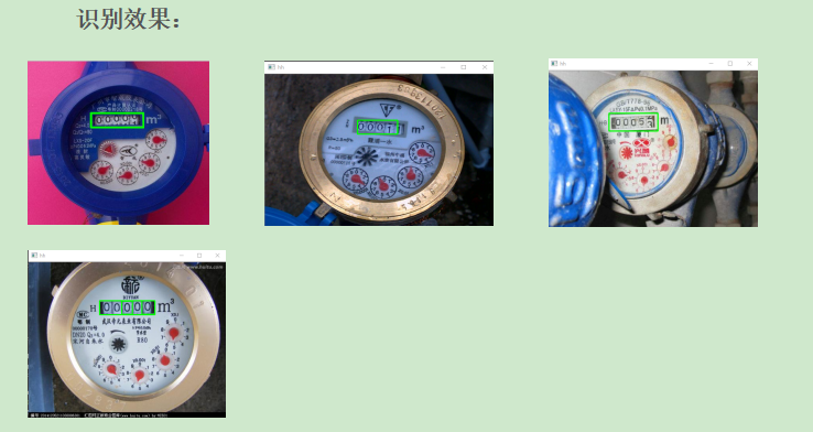
# -*- coding: utf-8 -*-
"""
Created on Tue Sep 17 19:00:45 2019

@author: xxr
"""
from cv2 import cv2  #因为cv2里面还有cv2 所以要这样干！
import numpy as np  


#读取原始图片
image= cv2.imread('shuibiao1.jpg')

#图片的缩小，记住比例 的缩放 
r = 500.0 / image.shape[1]
dim = (500, int(image.shape[0] * r))
image = cv2.resize(image, dim, interpolation = cv2.INTER_AREA)
#图像灰度化处理
grayImage = cv2.cvtColor(image,cv2.COLOR_BGR2GRAY)
#基于Canny的边沿检测(生成的也是二值图)
canny=cv2.Canny(grayImage,30,180)
cv2.imshow('canny', canny)
# 运用OpenCV findContours函数检测图像所有轮廓
contours, hierarchy = cv2.findContours(canny,cv2.RETR_CCOMP,cv2.CHAIN_APPROX_SIMPLE)
# 对于检测出的轮廓，contourArea限制轮廓所包围的面积的大小,boundingRect识别出正矩形，通过矩形的宽度和高度筛选出想要的图片区域。
# count=0
# minx=10000
# miny=10000
# height=0
# weight=0
for cnt in contours:
    if cv2.contourArea(cnt)>800:  #筛选出面积大于30的轮廓
        [x,y,w,h] = cv2.boundingRect(cnt) #x,y是左上角的坐标，h,w是高和宽
        if  h > 28 and h < 50:  # 根据期望获取区域，即数字区域的实际高度预估28至50之间
            # if(minx>x):
            #     minx=x
            # if(miny>y):
            #     miny=y
            # count+=1
            # height+=h
            # weight+=w
            cv2.rectangle(image,(x,y),(x+w,y+h),(0,255,0),2)
#             #截取特定区域
# imagehh = image[miny:miny+height,minx:minx+weight]

cv2.imshow("hh",image)
# print(str(count)+"jjjjjjjj")




cv2.waitKey(0)
cv2.destroyAllWindows()

对水表图片进行的hough（霍夫）直线检测

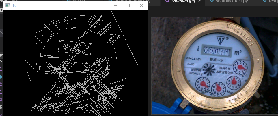
  1 # -*- coding: utf-8 -*-
  2 """
  3 Created on Tue Sep 17 19:00:45 2019
  4 
  5 @author: xxr
  6 """
  7 from cv2 import cv2  #因为cv2里面还有cv2 所以要这样干！
  8 import numpy as np  
  9 
 10 #读取原始图片
 11 image= cv2.imread('shuibiao.jpg')
 12 
 13 #读入一张白色的图
 14 image2=cv2.imread('white.png')
 15 image3=image2
 16 
 17 #图片的缩小，记住比例 的缩放 
 18 r = 500.0 / image.shape[1]
 19 dim = (500, int(image.shape[0] * r))
 20 image = cv2.resize(image, dim, interpolation = cv2.INTER_AREA)
 21 image2=cv2.resize(image2, dim, interpolation = cv2.INTER_AREA)
 22 
 23 #图像灰度化处理
 24 grayImage = cv2.cvtColor(image,cv2.COLOR_BGR2GRAY)
 25 #基于Canny的边沿检测(生成的也是二值图)
 26 canny=cv2.Canny(grayImage,30,180)
 27 #cv2.imshow("canny_image",canny)
 28 #再canny处理图像以后 用hough直线检测
 29 #统计概率霍夫线变换
 30 
 31 
 32                                #  步长         阈值      最小直线长度    最大构成直线的点的间隔
 33 lines = cv2.HoughLinesP(canny, 1, np.pi / 180, 60, minLineLength=30, maxLineGap=8)
 34 for line in lines:
 35         x1, y1, x2, y2 = line[0]
 36         cv2.line(image2, (x1, y1), (x2, y2), (0, 0, 255), 1)
 37 
 38 
 39 
 40 #这里进行矩形的轮廓检测  !!!应该找 白色的矩形框
 41 image2 = cv2.cvtColor(image2,cv2.COLOR_BGR2GRAY)
 42 #黑白颜色颠倒
 43 height, width = image2.shape
 44 dst = np.zeros((height,width,1), np.uint8)
 45 for i in range(0, height):
 46     for j in range(0, width):
 47         grayPixel = image2[i, j]
 48         dst[i, j] = 255-grayPixel
 49 
 50 
 51 #高斯滤波（使图像模糊，平滑）
 52 #dst=cv2.GaussianBlur(dst,(7,7),0)
 53 
 54 cv2.imshow('dst', dst)
 55 contours, hierarchy = cv2.findContours(dst,cv2.RETR_CCOMP,cv2.CHAIN_APPROX_SIMPLE)
 56 
 57 # #绘制直线
 58 # max=0
 59 # max_i=0
 60 # print(len(contours[2]))
 61 # for i in range(len(contours)):
 62 #         if(5==len(contours[i])):
 63 #                 max_i=i
 64 # cv2.drawContours(image3,contours,-1,(0,255,255),3)
 65 # cv2.imshow("draw_img0", image3)
 66 
 67 # #绘制矩形
 68 # for i in range(0,len(contours)):  
 69 #     x, y, w, h = cv2.boundingRect(contours[i])   
 70 #     cv2.rectangle(image3, (x,y), (x+w,y+h), (153,153,0), 5) 
 71 #cv2.imshow("draw_img0", image3)
 72 
 73 #打印矩形
 74 # for i in range(0,len(contours)):  
 75 #     x, y, w, h = cv2.boundingRect(contours[i])
 76 #     print(contours[0])  
 77 #     cv2.rectangle(image3, (x,y), (x+w,y+h), (255,153,0), 5) 
 78 
 79 #标准霍夫线变换（但在这里不太实用）
 80 # lines = cv2.HoughLines(canny, 1, np.pi/180, 150)
 81 # for line in lines:
 82 #         rho, theta = line[0]  #line[0]存储的是点到直线的极径和极角，其中极角是弧度表示的。
 83 #         a = np.cos(theta)   #theta是弧度
 84 #         b = np.sin(theta)
 85 #         x0 = a * rho    #代表x = r * cos（theta）
 86 #         y0 = b * rho    #代表y = r * sin（theta）
 87 #         x1 = int(x0 + 1000 * (-b)) #计算直线起点横坐标
 88 #         y1 = int(y0 + 1000 * a)    #计算起始起点纵坐标
 89 #         x2 = int(x0 - 1000 * (-b)) #计算直线终点横坐标
 90 #         y2 = int(y0 - 1000 * a)    #计算直线终点纵坐标    注：这里的数值1000给出了画出的线段长度范围大小，数值越小，画出的线段越短，数值越大，画出的线段越长
 91 #         cv2.line(image, (x1, y1), (x2, y2), (0, 0, 255), 2)    #点的坐标必须是元组，不能是列表。
 92 # cv2.imshow("image-lines", image)
 93 
 94 # 二值化图片
 95 # #自适应阈值化能够根据图像不同区域亮度分布，改变阈值
 96 # #threshold_pic =  cv2.adaptiveThreshold(grayImage, 255, cv2.ADAPTIVE_THRESH_GAUSSIAN_C,cv2.THRESH_BINARY, 25, 10)
 97 # ret,threshold_pic=cv2.threshold(grayImage,127, 255, cv2.THRESH_BINARY)
 98 # cv2.imshow("threshold_image",threshold_pic)
 99 #等待显示（不添加这两行将会报错）
100 cv2.waitKey(0)
101 cv2.destroyAllWindows()

# -*- coding: utf-8 -*-
"""
Created on Tue Sep 17 19:00:45 2019

@author: xxr
"""
from cv2 import cv2  #因为cv2里面还有cv2 所以要这样干！
import numpy as np  

#读取原始图片
image= cv2.imread('shuibiao.jpg')

#读入一张白色的图
image2=cv2.imread('white.png')
image3=image2

#图片的缩小，记住比例 的缩放 
r = 500.0 / image.shape[1]
dim = (500, int(image.shape[0] * r))
image = cv2.resize(image, dim, interpolation = cv2.INTER_AREA)
image2=cv2.resize(image2, dim, interpolation = cv2.INTER_AREA)

#图像灰度化处理
grayImage = cv2.cvtColor(image,cv2.COLOR_BGR2GRAY)
#基于Canny的边沿检测(生成的也是二值图)
canny=cv2.Canny(grayImage,30,180)
#cv2.imshow("canny_image",canny)
#再canny处理图像以后 用hough直线检测
#统计概率霍夫线变换


                               #  步长         阈值      最小直线长度    最大构成直线的点的间隔
lines = cv2.HoughLinesP(canny, 1, np.pi / 180, 60, minLineLength=30, maxLineGap=8)
for line in lines:
        x1, y1, x2, y2 = line[0]
        cv2.line(image2, (x1, y1), (x2, y2), (0, 0, 255), 1)



#这里进行矩形的轮廓检测  !!!应该找 白色的矩形框
image2 = cv2.cvtColor(image2,cv2.COLOR_BGR2GRAY)
#黑白颜色颠倒
height, width = image2.shape
dst = np.zeros((height,width,1), np.uint8)
for i in range(0, height):
    for j in range(0, width):
        grayPixel = image2[i, j]
        dst[i, j] = 255-grayPixel


#高斯滤波（使图像模糊，平滑）
#dst=cv2.GaussianBlur(dst,(7,7),0)

cv2.imshow('dst', dst)
contours, hierarchy = cv2.findContours(dst,cv2.RETR_CCOMP,cv2.CHAIN_APPROX_SIMPLE)

# #绘制直线
# max=0
# max_i=0
# print(len(contours[2]))
# for i in range(len(contours)):
#         if(5==len(contours[i])):
#                 max_i=i
# cv2.drawContours(image3,contours,-1,(0,255,255),3)
# cv2.imshow("draw_img0", image3)

# #绘制矩形
# for i in range(0,len(contours)):  
#     x, y, w, h = cv2.boundingRect(contours[i])   
#     cv2.rectangle(image3, (x,y), (x+w,y+h), (153,153,0), 5) 
#cv2.imshow("draw_img0", image3)

#打印矩形
# for i in range(0,len(contours)):  
#     x, y, w, h = cv2.boundingRect(contours[i])
#     print(contours[0])  
#     cv2.rectangle(image3, (x,y), (x+w,y+h), (255,153,0), 5) 

#标准霍夫线变换（但在这里不太实用）
# lines = cv2.HoughLines(canny, 1, np.pi/180, 150)
# for line in lines:
#         rho, theta = line[0]  #line[0]存储的是点到直线的极径和极角，其中极角是弧度表示的。
#         a = np.cos(theta)   #theta是弧度
#         b = np.sin(theta)
#         x0 = a * rho    #代表x = r * cos（theta）
#         y0 = b * rho    #代表y = r * sin（theta）
#         x1 = int(x0 + 1000 * (-b)) #计算直线起点横坐标
#         y1 = int(y0 + 1000 * a)    #计算起始起点纵坐标
#         x2 = int(x0 - 1000 * (-b)) #计算直线终点横坐标
#         y2 = int(y0 - 1000 * a)    #计算直线终点纵坐标    注：这里的数值1000给出了画出的线段长度范围大小，数值越小，画出的线段越短，数值越大，画出的线段越长
#         cv2.line(image, (x1, y1), (x2, y2), (0, 0, 255), 2)    #点的坐标必须是元组，不能是列表。
# cv2.imshow("image-lines", image)

# 二值化图片
# #自适应阈值化能够根据图像不同区域亮度分布，改变阈值
# #threshold_pic =  cv2.adaptiveThreshold(grayImage, 255, cv2.ADAPTIVE_THRESH_GAUSSIAN_C,cv2.THRESH_BINARY, 25, 10)
# ret,threshold_pic=cv2.threshold(grayImage,127, 255, cv2.THRESH_BINARY)
# cv2.imshow("threshold_image",threshold_pic)
#等待显示（不添加这两行将会报错）
cv2.waitKey(0)
cv2.destroyAllWindows()