周志华西瓜书习题3.3

做这道题花费了五天左右的时间，主要是python基础不怎么样，看着别人的代码，主要是参考https://blog.csdn.net/Snoopy_Yuan/article/details/63684219

一行一行地弄懂，然后再自己写。

一、获得以下经验：

1、在使用梯度下降算法求解数值的最优解时，要观察拟合曲线的拟合情况，拟合曲线逼近稳定值才可

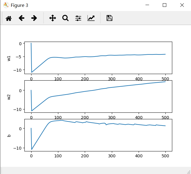
在上图所示的拟合曲线中，曲线没有趋于稳定，应调节梯度下降的步长，或者增加拟合次数，

调节后的拟合结果如下图

拟合曲线趋于稳定值，拟合效果还是比较好的（巧了，在拟合500次的情况下步长比它大，比它小的都不稳定，但增大拟合次数可解决这一问题）

二、源代码

源代码的算法部分是在看懂别人的代码的基础上自己敲的，其余部分直接从https://blog.csdn.net/Snoopy_Yuan/article/details/63684219摘的，希望原作者不要骂我。。。。。。。

1、主程序 main_self.py

 1 import numpy as np  # for matrix calculation
 2 
 3 import matplotlib.pyplot as plt
 4 
 5 # load the CSV file as a numpy matrix
 6 
 7 dataset = np.loadtxt('../watermelon_3a.csv', delimiter=",") #以逗号为分隔符，读取文件数据，读出一个17行四列的数组
 8 
 9 # separate the data from the target attributes
10 
11 X = dataset[:, 1:3]#截取第一列，第二列数据
12 
13 y = dataset[:, 3]#截取第三列数据
14 
15 m, n = np.shape(X)#m反回行数，n反回列数
16 
17 # draw scatter diagram to show the raw data
18 
19 f1 = plt.figure(1)
20 
21 plt.title('watermelon_3a')
22 
23 plt.xlabel('density')
24 
25 plt.ylabel('ratio_sugar')
26 
27 plt.scatter(X[y == 0, 0], X[y == 0, 1], marker='o', color='k', s=100, label='bad')
28 #X[y == 0, 0]是一个一行九列的向量[0.666 0.243 0.245 0.343 0.639 0.657 0.36  0.593 0.719]，它取得是X矩阵的第0列中，对y==0为真的行数的数据
29 #scatter函数是用来绘制散点图的 https://blog.csdn.net/fei347795790/article/details/94331112
30 
31 plt.scatter(X[y == 1, 0], X[y == 1, 1], marker='o', color='g', s=100, label='good')
32 
33 plt.legend(loc='upper right')
34 
35 #plt.show()#用来显示图像   #如果不把这一行注释掉，程序执行到此处自动结束
36 
37 
38 from sklearn import model_selection
39 
40 #import self_def
41 import self_def_xdl
42 
43 # X_train, X_test, y_train, y_test
44 
45 np.ones(n)
46 
47 m, n = np.shape(X)
48 
49 X_ex = np.c_[X, np.ones(m)]  # extend the variable matrix to [x, 1]  为啥要写成X_ex呢，在p59 式3.25下面
50 
51 X_train, X_test, y_train, y_test = model_selection.train_test_split(X_ex, y, test_size=0.5, random_state=0)#划分训练集和测试集
52 
53 # using gradDescent to get the optimal parameter beta = [w, b] in page-59
54 
55 beta = self_def_xdl.gradDscent(X_train, y_train)#beta = -4.7 0.3 2.5
56 
57 # prediction, beta mapping to the model
58 
59 y_pred = self_def_xdl.predict(X_test, beta)
60 
61 m_test = np.shape(X_test)[0]
62 
63 # calculation of confusion_matrix and prediction accuracy计算混淆矩阵和计算的准确性
64 
65 cfmat = np.zeros((2, 2))
66 
67 for i in range(m_test):
68 
69     if y_pred[i] == y_test[i] == 0:
70         cfmat[0, 0] += 1
71 
72     elif y_pred[i] == y_test[i] == 1:
73         cfmat[1, 1] += 1
74 
75     elif y_pred[i] == 0:
76         cfmat[1, 0] += 1
77 
78     elif y_pred[i] == 1:
79         cfmat[0, 1] += 1
80 
81 print(cfmat)

二、自定义函数 self_def_xdl.py

  1 def likelihood_xdl(X,y,beta):
  2     '''
  3     对应于实现P59-3.29
  4     :param X:(x;1) m行n+1列的数组，n列代表样本有n个维度，m行代表有m个样本，为啥要n+1列呢，见3.25下面的一段话
  5     :param y: m行1列的数组
  6     :param beta: 1行n+1列的数组beta = (w；b)
  7     :return: l_beta，一个数值
  8     '''
  9     import numpy as np
 10     m,n = np.shape(X)
 11     sum = 0
 12     for i in range(m):
 13         sum += -y[i]*np.dot(beta,X[i].T)+np.math.log(1+np.math.exp(np.dot(beta,X[i].T)))
 14     return sum
 15 
 16 def gradDscent(X,y):
 17     '''
 18     我使用的是批量梯度下降算法，如果样本的数据量比较大，还可使用随机梯度下降算法，详见https://blog.csdn.net/lilyth_lilyth/article/details/8973972
 19     X,y是训练集的数据，对3.27式使用梯度下降算法
 20     :param X: (x;1) m行n+1列的数组，n列代表样本有n个维度，m行代表有m个样本，为啥要n+1列呢，见3.25下面的一段话
 21     :param y: m行1列的数组
 22     :return:经过梯度下降算法一步一步迭代得出的beta
 23     '''
 24     import numpy as np
 25     import matplotlib.pyplot as plt
 26     m,n = np.shape(X)
 27     h = 0.11#步长
 28     beta = np.zeros(n)#1行n列
 29     delta_beta = h*np.ones(n)
 30     max_times = 1500#迭代次数
 31     beta_history = np.zeros((n,max_times))#记录beta的历史数据 #注意，括号中还有括号 #注意n和maxtime的顺序
 32     l_beta = 0
 33     l_beta_temp = 0
 34 
 35     for i in range(max_times):
 36         temp_beta = beta #暂存beta数据
 37         beta_history[:, i] = beta.T  # 记录下beta的历史，后面去查看拟合情况
 38         for j in range(n):
 39             beta[j] += delta_beta[j]
 40 
 41             l_beta_temp = likelihood_xdl(X,y,beta)
 42             delta_beta[j] = -h*(l_beta_temp-l_beta)/delta_beta[j]#使用式B.16,B.17更新delta_beta
 43 
 44             beta = temp_beta#恢复beta的数据
 45 
 46         beta += delta_beta
 47         l_beta = likelihood_xdl(X,y,beta)
 48 
 49     t = np.arange(max_times)
 50     f3 = plt.figure(3)
 51     p1 = plt.subplot(311)  # 311-3行1列第一个
 52     p1.plot(t, beta_history[0])
 53 
 54     plt.ylabel('w1')
 55 
 56     p2 = plt.subplot(312)
 57 
 58     p2.plot(t, beta_history[1])
 59 
 60     plt.ylabel('w2')
 61 
 62     p3 = plt.subplot(313)
 63 
 64     p3.plot(t, beta_history[2])
 65 
 66     plt.ylabel('b')
 67 
 68     plt.show()  # 显示所有图像
 69 
 70     return beta
 71 
 72 def sigmoid(x, beta):
 73     '''
 74     式3.18和3.25下面的一段话
 75     @param x: 测试集的一个样本，为一维行向量
 76 
 77     @param beta: 一维行向量
 78 
 79     @return: sigmoid函数预测结果
 80 
 81     '''
 82     import numpy as np
 83     return 1.0 / (1 + np.math.exp(- np.dot(beta, x.T)))
 84 
 85 
 86 def predict(X, beta):
 87     '''
 88 
 89     使用3.16式
 90 
 91     @param X: data sample form like [x, 1]
 92 
 93     @param beta: the parameter of sigmoid form like [w, b]
 94 
 95     @return: the class lable array
 96 
 97     '''
 98     import numpy as np
 99     m, n = np.shape(X)
100 
101     y = np.zeros(m)
102 
103     for i in range(m):
104 
105         if sigmoid(X[i], beta) > 0.5: y[i] = 1;
106 
107     return y
108 
109     return beta

三、原始数据集 watermelon_3a.csv

1,0.697,0.46,1
2,0.774,0.376,1
3,0.634,0.264,1
4,0.608,0.318,1
5,0.556,0.215,1
6,0.403,0.237,1
7,0.481,0.149,1
8,0.437,0.211,1
9,0.666,0.091,0
10,0.243,0.0267,0
11,0.245,0.057,0
12,0.343,0.099,0
13,0.639,0.161,0
14,0.657,0.198,0
15,0.36,0.37,0
16,0.593,0.042,0
17,0.719,0.103,0