为了更直观地说明光滑参数![]() 的变化对回归函数估计效果的影响,下面给出一个数值模拟例子。
的变化对回归函数估计效果的影响,下面给出一个数值模拟例子。
设有回归模型 ![]()
#模拟数据
n = 201
x = seq(0,2,0.01)
e = rnorm(n,0,0.2)
y = 2*x + sin(5*pi * x)+e
#局部常数拟合
#h = 0.1
plot(x,y,main = "h = 0.1")
lines(x,2*x + sin(5*pi * x),lty = 1,lwd = 1)#真实曲线
lines(lowess(x,y,f=0.1),pch = 1,lwd = 2)#lowess
data = as.data.frame(cbind(x,y))
model1 = loess(y~x,data,span = 0.1,degree = 0)#loess
lines(x,model1$fit,col = "red")
legend(0.05,4.5,c("真实曲线","lowess fit","loess fit"),lty = 1,lwd = c(1,2,1),col = c(1,1,"red"))#加标签
#h = 0.05
plot(x,y,main = "h = 0.05")
lines(x,2*x + sin(5*pi * x),lty = 1,lwd = 1)#真实曲线
lines(lowess(x,y,f=0.05),pch = 1,lwd = 2)#lowess
model1 = loess(y~x,data,span = 0.05,degree = 0)#loess
lines(x,model1$fit,col = "red")
legend(0.05,4.5,c("真实曲线","lowess fit","loess fit"),lty = 1,lwd = c(1,2,1),col = c(1,1,"red"))#加标签
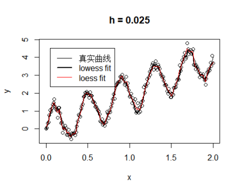
#h = 0.025
plot(x,y,main = "h = 0.025")
lines(x,2*x + sin(5*pi * x),lty = 1,lwd = 1)#真实曲线
lines(lowess(x,y,f=0.025),pch = 1,lwd = 2)#lowess
model1 = loess(y~x,data,span = 0.025,degree = 0)#loess
lines(x,model1$fit,col = "red")
legend(0.05,4.5,c("真实曲线","lowess fit","loess fit"),lty = 1,lwd = c(1,2,1),col = c(1,1,"red"))#加标签
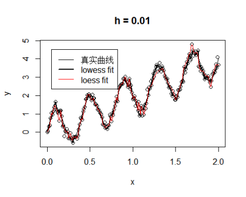
#h = 0.01
plot(x,y,main = "h = 0.01")
lines(x,2*x + sin(5*pi * x),lty = 1,lwd = 1)#真实曲线
lines(lowess(x,y,f=0.01),pch = 1,lwd = 2)#lowess
model1 = loess(y~x,data,span = 0.01,degree = 0)#loess
lines(x,model1$fit,col = "red")
legend(0.05,4.5,c("真实曲线","lowess fit","loess fit"),lty = 1,lwd = c(1,2,1),col = c(1,1,"red"))#加标签


有两个函数可以做局部加权回归:
1. lowess(x,y,f = )
f代表窗宽参数,f越大,则拟合曲线越光滑。
2. loess(formula,data,span,degree,…)
loess函数要比lowess函数强大,span是用来控制光滑度的,span越大则拟合曲线越光滑。lowess的参数f与loess的参数span代表含义并不相同。loess函数的参数degree是用来控制使用的多项式的阶数,一般可以选择1或2。(注意,当上面degree参数取0,图像显示lowess与loess拟合的结果是相似的)