如何理解高斯过程

A Visual Exploration of Gaussian Processes

地址：https://www.jgoertler.com/visual-exploration-gaussian-processes/

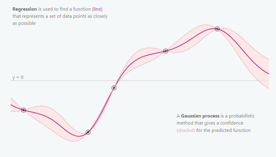
高斯过程是一种非参数建模方法，试图寻找与观测数据点相一致的所有可能函数的分布。

与所有贝叶斯方法相同，高斯过程从一个先验分布开始，并采用观测数据对其更新，从而得到函数的后验分布。

非参数方法并不是没有参数，而是有无穷多个参数（即，我们考虑的是函数的分布，可以含有任意多个参数。）。

核心思想

高斯过程从一个函数的先验分布开始，并采用观测数据对其更新，从而得到函数的后验分布。

如何表示函数的分布？听起来有些困难！事实证明，我们只需要在一个有限但任意的点集上（如，x1, x2, ..., xN）定义一个分布。

高斯过程假设是一个多变量联合高斯分布, 均值向量为

协方差矩阵通过一个被称为核函数K的东西进行计算。核函数是正定的，其形式有很多（参考Rasmussen and Williams book.）。

核函数应保证计算出的协方差矩阵满足对称半正定的性质。

其核心思想为，如果xi和xj被核函数认为是相似的，那么我们期望函数在这些点上的输出值也是相似的。

GPs的数学关键是多变量高斯分布。

我们是如何得出后验分布的？

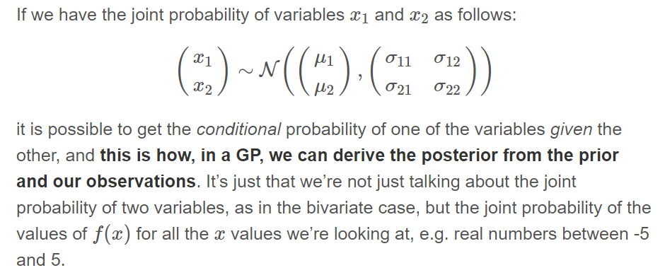
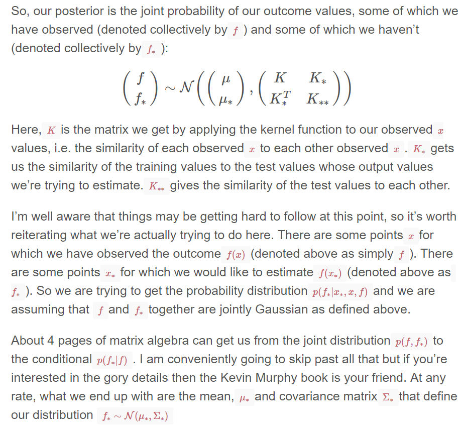
GPs的数学关键是多变量高斯分布。如果我们知道多变量的联合概率密度分布，在给定其他变量的情况下，有可能得到其中一个变量的条件概率，

这就是在gp中，我们如何从先验分布和我们的观测点中得出后验分布。

一个例子

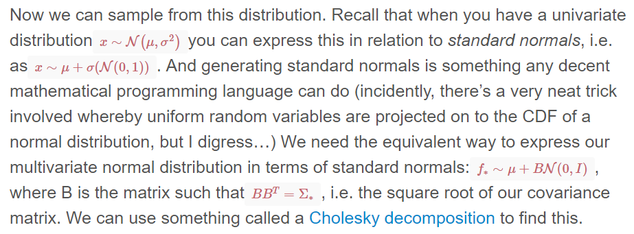
import numpy as np
import matplotlib.pyplot as pl

# Test data
n = 50
Xtest = np.linspace(-5, 5, n).reshape(-1,1)

# Define the kernel function
def kernel(a, b, param):
    sqdist = np.sum(a**2,1).reshape(-1,1) + np.sum(b**2,1) - 2*np.dot(a, b.T)
    return np.exp(-.5 * (1/param) * sqdist)

param = 0.1
K_ss = kernel(Xtest, Xtest, param)

# Get cholesky decomposition (square root) of the
# covariance matrix
L = np.linalg.cholesky(K_ss + 1e-15*np.eye(n))
# Sample 3 sets of standard normals for our test points,
# multiply them by the square root of the covariance matrix
f_prior = np.dot(L, np.random.normal(size=(n,3)))

# Now let's plot the 3 sampled functions.
pl.plot(Xtest, f_prior)
pl.axis([-5, 5, -3, 3])
pl.title('Three samples from the GP prior')
pl.show()

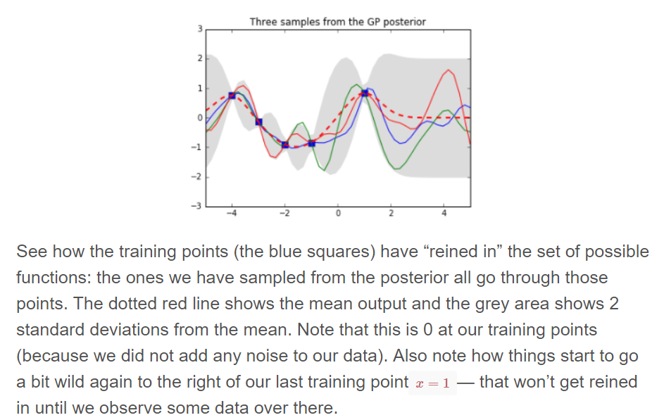
# Noiseless training data
Xtrain = np.array([-4, -3, -2, -1, 1]).reshape(5,1)
ytrain = np.sin(Xtrain)

# Apply the kernel function to our training points
K = kernel(Xtrain, Xtrain, param)
L = np.linalg.cholesky(K + 0.00005*np.eye(len(Xtrain)))

# Compute the mean at our test points.
K_s = kernel(Xtrain, Xtest, param)
Lk = np.linalg.solve(L, K_s)
mu = np.dot(Lk.T, np.linalg.solve(L, ytrain)).reshape((n,))

# Compute the standard deviation so we can plot it
s2 = np.diag(K_ss) - np.sum(Lk**2, axis=0)
stdv = np.sqrt(s2)
# Draw samples from the posterior at our test points.
L = np.linalg.cholesky(K_ss + 1e-6*np.eye(n) - np.dot(Lk.T, Lk))
f_post = mu.reshape(-1,1) + np.dot(L, np.random.normal(size=(n,3)))

pl.plot(Xtrain, ytrain, 'bs', ms=8)
pl.plot(Xtest, f_post)
pl.gca().fill_between(Xtest.flat, mu-2*stdv, mu+2*stdv, color="#dddddd")
pl.plot(Xtest, mu, 'r--', lw=2)
pl.axis([-5, 5, -3, 3])
pl.title('Three samples from the GP posterior')
pl.show()

如何理解高斯过程

A Visual Exploration of Gaussian Processes

核心思想

我们是如何得出后验分布的？

一个例子

Further Reading