机器翻译注意力机制及其PyTorch实现

前面阐述注意力理论知识,后面简单描述PyTorch利用注意力实现机器翻译

Effective Approaches to Attention-based Neural Machine Translation

简介

Attention介绍

在翻译的时候,选择性的选择一些重要信息。详情看这篇文章 。

本着简单和有效的原则,本论文提出了两种注意力机制

Global

每次翻译时,都选择关注所有的单词。和Bahdanau的方式 有点相似,但是更简单些。简单原理介绍

Local

每次翻译时,只选择关注一部分的单词。介于soft和hard注意力之间。(soft和hard见别的论文)。

优点有下面几个

  • 比Global和Soft更好计算
  • 局部注意力 随处可见、可微,更好实现和训练。

应用范围

在训练神经网络的时候,注意力机制应用十分广泛。让模型在不同的形式之间,学习对齐等等。有下面一些领域:

  • 机器翻译
  • 语音识别
  • 图片描述
  • between image objects and agent actions in the dynamic control problem (不懂,以后再说吧)

神经机器翻译

思想

输入句子x=(x1,x2,,xn)x=(x1,x2,⋯,xn) ,输出目标句子y=(y1,y2,,ym)y=(y1,y2,⋯,ym) 。

神经机器翻译(Neural machine translation, NMT),利用神经网络,直接对p(yx)p(y∣x) 进行建模。一般由Encoder和Decoder构成。Encoder-Decoder介绍文章链接 。

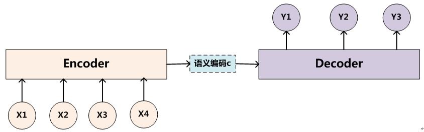
Encoder把输入句子xx 编码成一个语义向量ss (c表示也可以),然后由Decoder 一个一个产生目标单词 yiyilogp(yx)=mj=1logp(yjy<j,s)=mj=1logp(yjy1,,yj1,s)log⁡p(y∣x)=∑j=1mlog⁡p(yj∣y<j,s)=∑j=1mlog⁡p(yj∣y1,⋯,yj−1,s)但是怎么选择Encoder和Decoder(RNN, CNN, GRU, LSTM),怎么去生成语义ss却有很多选择。

概率计算

结合Decoder上一时刻的隐状态hj1hj−1和encoder给的语义向量ss,通过函数ff ,就可以计算出当前的隐状态hjhj :hj=f(hj1,s)hj=f(hj−1,s)通过函数gg对当前隐状态hjhj进行转换,再softmax,就可以得到翻译的目标单词yiyi了(选概率最大的那个)。

gg一般是线性变换,维数变化是[1,h][1,vocab_size][1,h]→[1,vocab_size]。p(yjy<j,s)=softmaxg(hj)p(yj∣y<j,s)=softmaxg(hj)语义向量ss​ 会贯穿整个翻译的过程,每一步翻译都会使用到语义向量的内容,这就是注意力机制

本论文的模型

本论文采用stack LSTM的构建NMT系统。如下所示:
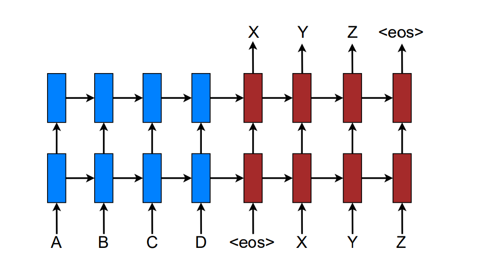
训练目标是Jt=(x,y)logp(yx)Jt=∑(x,y)−log⁡p(y∣x)

注意力模型

注意力模型广义上分为globallocal。Global的attention来自于整个序列,而local的只来自于序列的一部分。

解码总体流程

Decoder时,在时刻tt,要翻译出单词ytyt ,如下步骤:

  • 最顶层LSTM的隐状态 htht
  • 计算带有原句子信息语义向量ctct。Global和Local的区别在于ctct的计算方式不同
  • 串联ht,ctht,ct,计算得到带有注意力的隐状态 ^ht=tanh(Wc[ct;ht])h^t=tanh⁡(Wc[ct;ht])
  • 通过注意力隐状态得到预测概率 p(yty<t,x)=softmax(Ws^ht)p(yt∣y<t,x)=softmax(Wsh^t)

Global Attention

总体思路

在计算ctct 的时候,会考虑整个encoder的隐状态。Decoder当前隐状态htht, Encoder时刻s的隐状态¯hsh¯s。

对齐向量αtαt代表时刻tt 输入序列中的单词对当前单词ytyt 的对齐概率,长度是TxTx, 随着输入句子的长度而改变 。xsxs与ytyt 的对齐概率如下:αt(s)=align(ht,¯hs)=score(ht,¯hs)Txi=1score(ht,¯hi),softmaxαt(s)=align(ht,h¯s)=score(ht,h¯s)∑i=1Txscore(ht,h¯i),实际上softmax结合上面的解码总体流程,有下面的流程all(¯hs),htαtct.ct,ht^ht.^htytall(h¯s),ht→αt→ct.ct,ht→h^t.h^t→yt简单来说是htαtct^htytht→αt→ct→h^t→yt 。

score计算

score(ht,¯hs)score(ht,h¯s) 是一种基于内容content-based的函数,有3种实现方式score(ht,¯hs)=hTt¯hsdothTtWa¯hsgeneralvTatanh(Wa[ht;¯hs])concatscore(ht,h¯s)={htTh¯sdothtTWah¯sgeneralvaTtanh⁡(Wa[ht;h¯s])concat缺点

生成每个目标单词的时候,都必须注意所有的原单词, 这样计算量很大,翻译长序列可能很难,比如段落或者文章。

Local Attention

在生成目标单词的时候,Local会选择性地关注一小部分原单词去计算αt,ctαt,ct,这样就解决了Global的问题。如下图

Soft和Hard注意

Soft 注意 :类似global注意,权值会放在图片的所有patches中。计算复杂。

Hard 注意: 不同时刻,会选择不同的patch。虽然计算少,但是non-differentiable,并且需要复杂的技术去训练模型,比如方差减少和强化学习。

Local注意

类似于滑动窗口,计算一个对齐位置ptpt,根据经验设置窗口大小DD,那么需要注意的源单词序列是 :[ptD,pt+D][pt−D,pt+D]αtαt 的长度就是2D2D,只需要选择这2D2D个单词进行注意力计算,而不是Global的整个序列。

对齐位置选择

对齐位置的选择就很重要,主要有两种办法。

local-m (monotonic) 设置位置, 即以当前单词位置作为对齐位置pt=tpt=tlocal-p (predictive) 预测位置

SS 是输入句子的长度,预测对齐位置如下pt=Ssigmoid(vTptanh(Wpht)),pt[0,S]pt=S⋅sigmoid(vpTtanh⁡(Wpht)),pt∈[0,S]对齐向量计算

αtαt的长度就是2D2D,对于每一个s[ptD,pt+D]s∈[pt−D,pt+D], 为了更好地对齐,添加一个正态分布N(μ,σ2)N(μ,σ2),其中 μ=pt,σ=D2μ=pt,σ=D2。

计算对齐概率:αt(s)=align(ht,¯hs)exp((sμ)22σ2)=align(ht,¯hs)exp(2(spt)2D2)αt(s)=align(ht,h¯s)exp⁡(−(s−μ)22σ2)=align(ht,h¯s)exp⁡(−2(s−pt)2D2)

Input-feeding

前面的Global和Local两种方式中,在每一步的时候,计算每一个attention (实际上是指 ^hth^t),都是独立的,这样只是次最优的。

在每一步的计算中,这些attention应该有所关联,当前知道之前的attention才对。实际是应该有个coverage set去追踪之前的信息。

我们会把当前的注意^hth^t 作为下一次的输入,并且做一个串联,来计算新的attention,如下图所示

这样有两重意义:

  • 模型会知道之前的对齐选择
  • 会建立一个水平和垂直都很深的网络

PyTorch实现机器翻译

机器翻译github源代码

计算输入语义

比较简单,使用GRU进行编码,使用outputs作为哥哥句子的编码语义。PyTorch RNN处理变长序列

1
2
3
4
5
6
7
8
9
10
11
12
13
14
15
16
17
18
19
20
def forward(self, input_seqs, input_lengths, hidden=None):
''' 对输入的多个句子经过GRU计算出语义信息
1. input_seqs > embeded
2. embeded - packed > GRU > outputs - pad -output
Args:
input_seqs: [s, b]
input_lengths: list[int],每个batch句子的真实长度
Returns:
outputs: [s, b, h]
hidden: [n_layer, b, h]
'''
# 一次运行,多个batch,多个序列
embedded = self.embedding(input_seqs)
packed = nn.utils.rnn.pack_padded_sequence(embedded, input_lengths)
outputs, hidden = self.gru(packed, hidden)
outputs, output_length = nn.utils.rnn.pad_packed_sequence(outputs)
# 双向,两个outputs求和
if self.bidir is True:
outputs = outputs[:, :, :self.hidden_size] + outputs[:, :, self.hidden_size:]
return outputs, hidden

计算对齐向量

实际上就是attn_weights, 也就是输入序列对当前要预测的单词的一个注意力分配

输入输出定义

Encoder的输出,所有语义cc,encoder_outputs, [is, b, h]。 is=input_seq_len是输入句子的长度

当前时刻Decoder的htht, decoder_rnn_output, [ts, b, h] 。实际上ts=1, 因为每次解码一个单词

1
2
3
4
5
6
7
8
def forward(self, rnn_outputs, encoder_outputs):
'''ts个时刻,计算ts个与is的对齐向量,也是注意力权值
Args:
rnn_outputs -- Decoder中GRU的输出[ts, b, h]
encoder_outputs -- Encoder的最后的输出, [is, b, h]
Returns:
attn_weights -- Yt与所有Xs的注意力权值,[b, ts, is]
'''

计算得分

使用gerneral的方式,先过神经网络(线性层),再乘法计算得分

1
2
3
4
# 过Linear层 (b, h, is)
encoder_outputs = self.attn(encoder_outputs).transpose(1, 2)
# [b,ts,is] < [b,ts,h] * [b,h,is]
attn_energies = rnn_outputs.bmm(encoder_outputs)

softmax计算对齐向量

每一行都是原语义对于某个单词的注意力分配权值向量。对齐向量实际例子

1
2
3
# [b,ts,is]
attn_weights = my_log_softmax(attn_energies)
return attn_weights

计算新的语义

新的语义也就是,对于翻译单词wtwt所需要的带注意力的语义。

输入输出

1
2
3
4
5
6
7
8
9
10
11
12
13
14
15
16
17
def forward(self, input_seqs, last_hidden, encoder_outputs):
'''
一次输入(ts, b),b个句子, ts=target_seq_len
1. input > embedded
2. embedded, last_hidden --GRU-- rnn_output, hidden
3. rnn_output, encoder_outpus --Attn-- attn_weights
4. attn_weights, encoder_outputs --相乘-- context
5. rnn_output, context --变换,tanh,变换-- output
Args:
input_seqs: [ts, b] batch个上一时刻的输出的单词,id表示。每个batch1个单词
last_hidden: [n_layers, b, h]
encoder_outputs: [is, b, h]
Returns:
output: 最终的输出,[ts, b, o]
hidden: GRU的隐状态,[nl, b, h]
attn_weights: 对齐向量,[b, ts, is]
'''

当前时刻Decoder的隐状态

输入上一时刻的单词和隐状态,通过GRU,计算当前的隐状态。实际上ts=1

1
2
# (ts, b, h), (nl, b, h)
rnn_output, hidden = self.gru(embedded, last_hidden)

计算对齐向量

当前时刻的隐状态 rnn_output 和源句子的语义encoder_outputs,计算对齐向量。对齐向量

每一行都是原句子对当前单词(只有一行)的注意力分配。

1
2
3
4
# 对齐向量 [b,ts,is]
attn_weights = self.attn(rnn_output, encoder_outputs)
# 如
[0.1, 0.2, 0.7]

计算新的语义

原语义和原语义对当前单词分配的注意力,计算当前需要的新语义。

1
2
3
# 新的语义 
# [b,ts,h] < [b,ts,is] * [b,is,h]
context = attn_weights.bmm(encoder_outputs.transpose(0, 1))

预测当前单词

结合新语义和当前隐状态预测新单词

1
2
3
4
5
6
7
8
9
# 语义和当前隐状态结合 [ts, b, 2h] < [ts, b, h], [ts, b, h]
output_context = torch.cat((rnn_output, context), 2)
# [ts, b, h] 线性层2h-h
output_context = self.concat(output_context)
concat_output = F.tanh(output_context)
# [ts, b, o] 线性层h-o
output = self.out(concat_output)
output = my_log_softmax(output)
return output

总结

1
2
3
4
5
6
7
8
9
10
11
12
13
14
15
16
17
# 1. 对齐向量
# 过Linear层 (b, h, is)
encoder_outputs = self.attn(encoder_outputs).transpose(1, 2)

# 关联矩阵 [b,ts,is] < [b,ts,h] * [b,h,is]
attn_energies = rnn_outputs.bmm(encoder_outputs)
# 每一行求softmax [b,ts,is]
'''每一行都是原语义对当前单词的注意力分配向量'''
attn_weights = my_log_softmax(attn_energies)

# 2. 新语义
# 新的语义 [b,ts,h] < [b,ts,is] * [b,is,h]
context = attn_weights.bmm(encoder_outputs.transpose(0, 1))

# 3. 新语义和当前隐状态结合,输出
# 语义和输出 [ts, b, 2h] < [ts, b, h], [ts, b, h]
output_context = torch.cat((rnn_output, context), 2)
原文地址:https://www.cnblogs.com/jfdwd/p/11065998.html