- 分类树和回归树参数差别:
- criterion
- 分类:使用信息增益,
- 回归:
- 均方误差MSE,使用均值。mse是父节点与叶子节点之间的均方误差,用来选择特征。同时也是用于衡量模型质量的指标。均方误差是正的,但是sklearn中的均方误差是负数。
- 绝对误差mae,使用中值。
- 注意:回归树的接口score默认返回的是R方(负无穷到1,越接近1越好),不是mse
from sklearn.datasets import load_boston
from sklearn.model_selection import cross_val_score
from sklearn.ensemble import RandomForestRegressor
boston = load_boston()
import sklearn
sorted(sklearn.metrics.SCORERS.keys())
['accuracy',
 'adjusted_mutual_info_score',
 'adjusted_rand_score',
 'average_precision',
 'balanced_accuracy',
 'brier_score_loss',
 'completeness_score',
 'explained_variance',
 'f1',
 'f1_macro',
 'f1_micro',
 'f1_samples',
 'f1_weighted',
 'fowlkes_mallows_score',
 'homogeneity_score',
 'jaccard',
 'jaccard_macro',
 'jaccard_micro',
 'jaccard_samples',
 'jaccard_weighted',
 'max_error',
 'mutual_info_score',
 'neg_log_loss',
 'neg_mean_absolute_error',
 'neg_mean_squared_error',
 'neg_mean_squared_log_error',
 'neg_median_absolute_error',
 'normalized_mutual_info_score',
 'precision',
 'precision_macro',
 'precision_micro',
 'precision_samples',
 'precision_weighted',
 'r2',
 'recall',
 'recall_macro',
 'recall_micro',
 'recall_samples',
 'recall_weighted',
 'roc_auc',
 'v_measure_score']
regresor = RandomForestRegressor(n_estimators=100, random_state=0)
cross_val_score(regresor, boston.data, boston.target, cv=10
               , scoring="neg_mean_squared_error"  # 可以通过 sklearn.metrics.SCORERS.keys() 查看scoring对应的参数,默认是R方
               )
# 返回10次交叉验证的衡量指标结果
array([-10.72900447,  -5.36049859,  -4.74614178, -20.84946337,
       -12.23497347, -17.99274635,  -6.8952756 , -93.78884428,
       -29.80411702, -15.25776814])
用随机森林回归填补缺失值
import numpy as np
import pandas as pd
import matplotlib.pyplot as plt
from sklearn.datasets import load_boston
from sklearn.ensemble import RandomForestRegressor
from sklearn.model_selection import cross_val_score
dataset = load_boston()
dataset.data.shape
(506, 13)
x_full, y_full = dataset.data, dataset.target  # 保存完整的数据
n_samples = x_full.shape[0]
n_features = x_full.shape[1]
n_samples, n_features
(506, 13)
# 首先确定希望放入的缺失值数据的比例。
rng = np.random.RandomState(0)
missing_rate = 0.5
n_missing_samples = int(np.floor(n_samples * n_features * missing_rate))
n_missing_samples
3289
# 构建缺失数据

missing_features = rng.randint(0, n_features, n_missing_samples)  # 生成从0-n之间的n_missing_samples个数据
missing_samples = rng.randint(0, n_samples, n_missing_samples)

x_missing = x_full.copy()
y_missing = y_full.copy()

x_missing[missing_samples, missing_features] = np.nan
x_missing = pd.DataFrame(x_missing)
x_missing
| 0 | 1 | 2 | 3 | 4 | 5 | 6 | 7 | 8 | 9 | 10 | 11 | 12 | |
|---|---|---|---|---|---|---|---|---|---|---|---|---|---|
| 0 | NaN | 18.0 | NaN | NaN | 0.538 | NaN | 65.2 | 4.0900 | 1.0 | 296.0 | NaN | NaN | 4.98 |
| 1 | 0.02731 | 0.0 | NaN | 0.0 | 0.469 | NaN | 78.9 | 4.9671 | 2.0 | NaN | NaN | 396.90 | 9.14 |
| 2 | 0.02729 | NaN | 7.07 | 0.0 | NaN | 7.185 | 61.1 | NaN | 2.0 | 242.0 | NaN | NaN | NaN |
| 3 | NaN | NaN | NaN | 0.0 | 0.458 | NaN | 45.8 | NaN | NaN | 222.0 | 18.7 | NaN | NaN |
| 4 | NaN | 0.0 | 2.18 | 0.0 | NaN | 7.147 | NaN | NaN | NaN | NaN | 18.7 | NaN | 5.33 |
| ... | ... | ... | ... | ... | ... | ... | ... | ... | ... | ... | ... | ... | ... |
| 501 | NaN | NaN | NaN | 0.0 | 0.573 | NaN | 69.1 | NaN | 1.0 | NaN | 21.0 | NaN | 9.67 |
| 502 | 0.04527 | 0.0 | 11.93 | 0.0 | 0.573 | 6.120 | 76.7 | 2.2875 | 1.0 | 273.0 | NaN | 396.90 | 9.08 |
| 503 | NaN | NaN | 11.93 | NaN | 0.573 | 6.976 | 91.0 | NaN | NaN | NaN | 21.0 | NaN | 5.64 |
| 504 | 0.10959 | 0.0 | 11.93 | NaN | 0.573 | NaN | 89.3 | NaN | 1.0 | NaN | 21.0 | 393.45 | 6.48 |
| 505 | 0.04741 | 0.0 | 11.93 | 0.0 | 0.573 | 6.030 | NaN | NaN | 1.0 | NaN | NaN | 396.90 | 7.88 |
506 rows × 13 columns
from sklearn.impute import SimpleImputer  # 专门用于填补缺失值的类

# 使用均值填充
imp_mean = SimpleImputer(missing_values=np.nan, strategy='mean')
x_missing_mean = imp_mean.fit_transform(x_missing)
x_missing_mean = pd.DataFrame(x_missing_mean)
x_missing_mean
| 0 | 1 | 2 | 3 | 4 | 5 | 6 | 7 | 8 | 9 | 10 | 11 | 12 | |
|---|---|---|---|---|---|---|---|---|---|---|---|---|---|
| 0 | 3.627579 | 18.000000 | 11.163464 | 0.066007 | 0.538000 | 6.305921 | 65.2 | 4.090000 | 1.000000 | 296.000000 | 18.521192 | 352.741952 | 4.980000 |
| 1 | 0.027310 | 0.000000 | 11.163464 | 0.000000 | 0.469000 | 6.305921 | 78.9 | 4.967100 | 2.000000 | 405.935275 | 18.521192 | 396.900000 | 9.140000 |
| 2 | 0.027290 | 10.722951 | 7.070000 | 0.000000 | 0.564128 | 7.185000 | 61.1 | 3.856371 | 2.000000 | 242.000000 | 18.521192 | 352.741952 | 12.991767 |
| 3 | 3.627579 | 10.722951 | 11.163464 | 0.000000 | 0.458000 | 6.305921 | 45.8 | 3.856371 | 9.383871 | 222.000000 | 18.700000 | 352.741952 | 12.991767 |
| 4 | 3.627579 | 0.000000 | 2.180000 | 0.000000 | 0.564128 | 7.147000 | 67.4 | 3.856371 | 9.383871 | 405.935275 | 18.700000 | 352.741952 | 5.330000 |
| ... | ... | ... | ... | ... | ... | ... | ... | ... | ... | ... | ... | ... | ... |
| 501 | 3.627579 | 10.722951 | 11.163464 | 0.000000 | 0.573000 | 6.305921 | 69.1 | 3.856371 | 1.000000 | 405.935275 | 21.000000 | 352.741952 | 9.670000 |
| 502 | 0.045270 | 0.000000 | 11.930000 | 0.000000 | 0.573000 | 6.120000 | 76.7 | 2.287500 | 1.000000 | 273.000000 | 18.521192 | 396.900000 | 9.080000 |
| 503 | 3.627579 | 10.722951 | 11.930000 | 0.066007 | 0.573000 | 6.976000 | 91.0 | 3.856371 | 9.383871 | 405.935275 | 21.000000 | 352.741952 | 5.640000 |
| 504 | 0.109590 | 0.000000 | 11.930000 | 0.066007 | 0.573000 | 6.305921 | 89.3 | 3.856371 | 1.000000 | 405.935275 | 21.000000 | 393.450000 | 6.480000 |
| 505 | 0.047410 | 0.000000 | 11.930000 | 0.000000 | 0.573000 | 6.030000 | 67.4 | 3.856371 | 1.000000 | 405.935275 | 18.521192 | 396.900000 | 7.880000 |
506 rows × 13 columns
# 使用 0填充缺失值
imp_0 = SimpleImputer(missing_values=np.nan, strategy='constant', fill_value=0)
x_missing_0 = imp_0.fit_transform(x_missing)
x_missing_0 = pd.DataFrame(x_missing_0)
x_missing_0
| 0 | 1 | 2 | 3 | 4 | 5 | 6 | 7 | 8 | 9 | 10 | 11 | 12 | |
|---|---|---|---|---|---|---|---|---|---|---|---|---|---|
| 0 | 0.00000 | 18.0 | 0.00 | 0.0 | 0.538 | 0.000 | 65.2 | 4.0900 | 1.0 | 296.0 | 0.0 | 0.00 | 4.98 |
| 1 | 0.02731 | 0.0 | 0.00 | 0.0 | 0.469 | 0.000 | 78.9 | 4.9671 | 2.0 | 0.0 | 0.0 | 396.90 | 9.14 |
| 2 | 0.02729 | 0.0 | 7.07 | 0.0 | 0.000 | 7.185 | 61.1 | 0.0000 | 2.0 | 242.0 | 0.0 | 0.00 | 0.00 |
| 3 | 0.00000 | 0.0 | 0.00 | 0.0 | 0.458 | 0.000 | 45.8 | 0.0000 | 0.0 | 222.0 | 18.7 | 0.00 | 0.00 |
| 4 | 0.00000 | 0.0 | 2.18 | 0.0 | 0.000 | 7.147 | 0.0 | 0.0000 | 0.0 | 0.0 | 18.7 | 0.00 | 5.33 |
| ... | ... | ... | ... | ... | ... | ... | ... | ... | ... | ... | ... | ... | ... |
| 501 | 0.00000 | 0.0 | 0.00 | 0.0 | 0.573 | 0.000 | 69.1 | 0.0000 | 1.0 | 0.0 | 21.0 | 0.00 | 9.67 |
| 502 | 0.04527 | 0.0 | 11.93 | 0.0 | 0.573 | 6.120 | 76.7 | 2.2875 | 1.0 | 273.0 | 0.0 | 396.90 | 9.08 |
| 503 | 0.00000 | 0.0 | 11.93 | 0.0 | 0.573 | 6.976 | 91.0 | 0.0000 | 0.0 | 0.0 | 21.0 | 0.00 | 5.64 |
| 504 | 0.10959 | 0.0 | 11.93 | 0.0 | 0.573 | 0.000 | 89.3 | 0.0000 | 1.0 | 0.0 | 21.0 | 393.45 | 6.48 |
| 505 | 0.04741 | 0.0 | 11.93 | 0.0 | 0.573 | 6.030 | 0.0 | 0.0000 | 1.0 | 0.0 | 0.0 | 396.90 | 7.88 |
506 rows × 13 columns
# 使用 随机森林 填充缺失值
# 通过已有的 特征数据 和 标签信息来 回归预测 缺失的数据
# 先填充缺失较少的特征数据

x_missing_reg = x_missing.copy()
sortindex = np.argsort(x_missing_reg.isnull().sum(axis=0)).values  # 计算出特征空值数据,然后排序返回对应列的索引
sortindex
array([ 6, 12, 8, 7, 9, 0, 2, 1, 5, 4, 3, 10, 11], dtype=int64)
# 遍历,填补空值
for i in sortindex:
    df = x_missing_reg
    fillc = df.iloc[:, i]
    df = pd.concat([df.drop(i, axis=1), pd.DataFrame(y_full)], axis=1)

    df_0 = SimpleImputer(missing_values=np.nan
                        , strategy='constant'
                        , fill_value=0
                        ).fit_transform(df)

    y_train = fillc[fillc.notnull()]
    y_test = fillc[fillc.isnull()]
    x_train = df_0[y_train.index, :]
    x_test = df_0[y_test.index, :]

    rfc = RandomForestRegressor(n_estimators=100)
    rfc = rfc.fit(x_train, y_train)
    y_predict = rfc.predict(x_test)

    x_missing_reg.loc[x_missing_reg.loc[:, i].isnull(), i] = y_predict
# 对填补好的数据进行建模

X = [x_full, x_missing_mean, x_missing_0, x_missing_reg]

mse = []
std = []
for x in X:
    estimator = RandomForestRegressor(random_state=0, n_estimators=100)
    scores = cross_val_score(estimator, x, y_full, scoring='neg_mean_squared_error', cv=5).mean()
    mse.append(scores * -1)
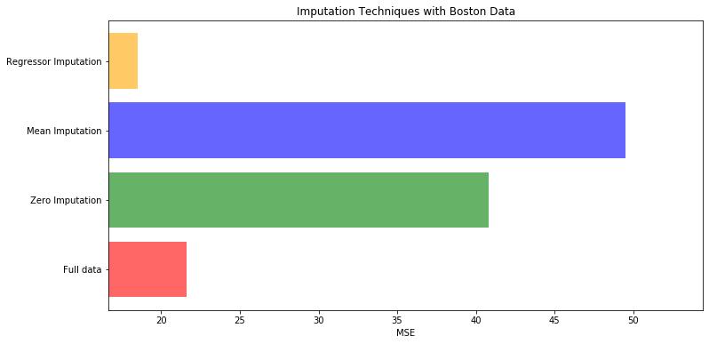
# 用所得的结果画出条形图

x_labels = ['Full data'
            , 'Zero Imputation'
            , 'Mean Imputation'
            , 'Regressor Imputation'
           ]
colors = ['r', 'g', 'b', 'orange']

plt.figure(figsize=(12, 6))
ax = plt.subplot(111)
for i in range(len(mse)):
    ax.barh(i, mse[i], color=colors[i], alpha=0.6, align='center')

ax.set_title('Imputation Techniques with Boston Data')
ax.set_xlim(left=np.min(mse) * 0.9,
            right=np.max(mse) * 1.1
           )
ax.set_yticks(range(len(mse)))
ax.set_xlabel('MSE')
ax.set_yticklabels(x_labels)
plt.show()