Everybody needs storage space nowadays. Whether it is used for high performance computing or simply storing family snapshots, we all need room to store data which is important to us.
In the old days (the 1990s) things were fairly easy: you had either ATA or SCSI. The much older RLL and MFM are now called ancient and therefore not talked about in this article. ATA was mainstream for about 10 years and SCSI was expensive, but also very fast. Both standards used a flatcable and the data was sent to and from the drive in parallel. But when speeds increased the timing of each of the separate signals became difficult and just like cd players in the 1980s manufacturers started using serial lines. This meant that higher speeds could be accomplished and also that the huge flatcables were now traded in for much smaller cable, which improved the airflow as well.
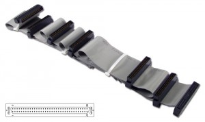
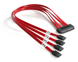
The pictures below show a long flat cable, containing 7 connectors as well as a (red) smaller 4 to 1 SAS or SATA cable.
RPM / IOps
In the beginning mainstream drives rotated at 3600 RPM where industry drives always were a bit ahead of these (5400). When the mainstream ones reached 5400, the industry reached 7200 and when mainstream reached 7200 the industry drives reached 10k and even 15k. Some mainstream SATA drives have 10k RPM, but these are rarely used except for the gaming community. The number of rotations per minute determines the number of IOps.
As a rule of thumb (ROT) the following list is commonly used (it’s a careful prediction of what drives actually can perform):
- 7200 RPM = 80 IOps
- 10k RPM = 130 IOps
- 15k RPM = 180 IOps
When IOs are smaller than used in the ROT (4 kB I believe it is) more IOps can be reached and when IOs are much larger, lower IOps are reached. The more I/Os per second a drive can handle, the faster the IOs are processed and your application can send or ask more data per second.
Command Queueing
Besides the number of rotations per minute the other main difference was that SCSI drives were faster because of added intelligence called Command Queueing (CQ). SCSI drives were able to change the order of IOs so the drive’s arms didn’t have to cross the whole surface to reach each block in the sequence they arrived in the drive and during a rotation movement of the arm was optimized to as many blocks could be addressed in as little rotations as possible. Two different CQ techniques were introduced: TCQ (Tagged Command Queueing) and NCQ (Native Command Queueing). You can think of Command Queueing like an elevator. The elevator goes up and down and people get in and out where they’re supposed to, but the elevator doesn’t follow the sequence of the people who pushed the buttons. If the elevator is going up, it keeps going up until it reaches the top and on the way down people can get in or out, but if a person needs to go up, he or she simply has to wait until the elevator goes up again.
With SCSI-2 the TCQ was introduced in the 90s and it was very commonly found on SCSI hard drives from then on. Since SCSI drives were mainly used in server hardware, TCQ was targeted to the enterprise-level hard drives.
The lack of CQ in the newer SATA drives in the early years of this millennium lead to a new CQ technique: NCQ. It was introduced with SATA-2 to provide home computers with the same benefit of IO reordering as the server drives already had for a decade.
In order to use NCQ or TCQ, both the hard drive port and the hard drive must support the standard. So, if you have a NCQ hard drive connector (the Serial ATA-2 ports found on most motherboards these days for example) but install a hard drive without this feature, you won’t notice any performance enhancement.
Command Queueing improves the performance of the hard drive when the computer sends a sequence of commands to read sectors distant from each other. The hard drive takes these commands and reorders them, in order to read the maximum possible data at just one rotation of the disk.
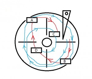
In the picture I tried to show what the elevator principle is. The computer asked the hard drive to read (or write) A, B, C and D blocks on the disk. Without any Command Queueing feature, the hard drive would take two and a half rotations of the disk to read all requested data (blue line). With Command Queuing, the hard drive will reorder the commands to B, D, A and C, taking only one rotation to read all requested data (red line).
NCQ can deal with up to 32 commands at a time, while TCQ can deal with up to 216 commands (TCQ hard drives, however, can usually support a queue of ”only“ 64 commands). TCQ also has two extra features over NCQ: the initiator (the computer, i.e., the port) can specify commands to be executed in the same order sent to the hard drive; and the initiator can send a high-priority command that will be executed before all other commands found in the queue.
So in short:
- NCQ = up to 32 commands
- TCQ = up to 216 commands (64 in general is used) + extra command priority features
So what else is there that differentiates SCSI, (P)ATA, SAS, NL-SAS and SATA?
Size matters
In part 1 we talked about Rotations Per Minute and Command Queuing, but what else is there that makes a certain drive a better choice than any other? Other differences are the size of the platters. Commonly used are 3.5 inch and 2.5 inch. Although it makes sense that smaller platters can rotate faster than larger platters in the end only the size of the drive cage matters. It’s in fact somewhat weird that most 2.5 inch drives now rotate at 10k RPM and the 3.5 inch drives at 15k. Being able to cool the device is probably the main reason why a 10k drive only spins at 10k RPM. If it would rotate any faster, it would heat up more and heat dissipation could become a serious problem. So if you need a high GB per square meter density and performance doesn’t really matter, then the 2.5 inch drives make sense, but if performance is the key differentiator, the more IOps you can squeeze out of each drive, the better. And since we’re not discussing data center designs here, only quality / performance counts.
Nowadays we only have a handful of drive interfaces:
- SAS
- NL-SAS
- SATA
- Fibe Channel
SAS and NL-SAS even share the same interface, in fact they’re the same drives, but the NL-SAS just rotates at 7200 RPM instead of 10k or 15k. FC drives still exist, but newer storage systems show that SAS is on the move and for FC it seems as if “the end is near”. So in fact only 2 species of drives remain:
- (NL-)SAS
- SATA
Since SAS is Serial Attached SCSI it uses TCQ and SATA uses NCQ. We already discussed both reordering mechanisms and TCQ has the advantage over NCQ.
Commonly available drive sizes (GB) are:
- SAS: 300, 600, 900 GB
- NL-SAS and SATA: 1, 2, 3 and 4 TB
Some additional sizes exist as well, but it’s the general idea that I am trying to point out here.
Speed of the interface
Since SAS and SATA are related, speeds of both interfaces are 1.5GBps, 3GBps or 6GBps. I even remember seeing Hitachi having a 12GBps drive already. But that’s just the speed of the interface. So data which comes in over the cable, entering the interface and the drive’s buffers will run at these speeds, but the rotating drives behind the interface become the limiting factor and these enormous speeds won’t be reached at all when large amounts of data are being transported. But short bursts of data will actually flow at speeds like this.
Single port / dual port
The SATA interface is half duplex and single ported, so there’s only 1 path from a controller to the drive. SAS is full duplex by design and can have dual ports as well. I say “can”, since it also requires 2 controllers to connect each drive and only the high end server controllers or storage arrays have this capability. So SAS drives with only a single port are being sold as well. In general you’ll find single ported drives in servers and dual ported drives in storage arrays.
So SAS drives offer higher speeds, although the drives spindels can only handle so many IOps, making them equally fast as SATA drives. Having dual ports does actually make SAS drives higher available, so in fact more reliable, since if one path goes down, the other could still be functional.
Durability / quality
So if only RPM differentiates SAS and SATA, having NL-SAS rotating at 7200 RPM and SATA rotating at 7200 RPM should make no difference, right? The only thing I can actually think of that might make sense is the quality of the drives.
- SATA/NL-SAS drives have a MTBF (Mean Time Between Failure) of 1.2 million hours. SAS drives have a MTBF of 1.6 million hours. SAS drives are more reliable than SATA when looking at MTBF.
- SATA drives have a BER (Bit Error Rate) of 1 read error in 10^15 bits read. SAS drives have a BER of 1 read error in 10^16 bits read. SAS drives are 10x more reliable for read errors. Keep in mind a read error is data loss without other mechanisms (RAID or Network RAID) in place to recover the data.
Conclusion
- If you want super performance, as well as quality, go for SAS running at 10k or 15k RPM
- If you want good quality and high capacity, go for NL-SAS running at 7200 RPM
- If you want cheap, mainstream high capacity storage, choose SATA running at 7200 RPM (or even lower speeds)