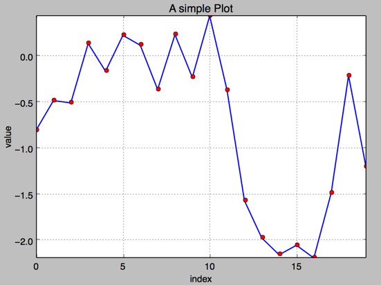
添加标题和标签 plt.title, plt.xlabe, plt.ylabel 离散点, 线
#!/etc/bin/python
#coding=utf-8
import numpy as np
import matplotlib as mpl
import matplotlib.pyplot as plt

np.random.seed(1000)
y = np.random.standard_normal(20)

plt.figure(figsize=(7,4)) #画布大小
plt.plot(y.cumsum(),'b',lw = 1.5) # 蓝色的线
plt.plot(y.cumsum(),'ro') #离散的点
plt.grid(True)
plt.axis('tight')
plt.xlabel('index')
plt.ylabel('value')
plt.title('A simple Plot')
plt.show()
np.random.seed(2000)
y = np.random.standard_normal((10, 2)).cumsum(axis=0)   #10行2列   在这个数组上调用cumsum 计算赝本数据在0轴(即第一维)上的总和
print y
b. 二维数据集
1.两个数据集绘图
#!/etc/bin/python
#coding=utf-8
import numpy as np
import matplotlib as mpl
import matplotlib.pyplot as plt

np.random.seed(2000)
y = np.random.standard_normal((10, 2))
plt.figure(figsize=(7,5))
plt.plot(y, lw = 1.5)
plt.plot(y, 'ro')
plt.grid(True)
plt.axis('tight')
plt.xlabel('index')
plt.ylabel('value')
plt.title('A simple plot')
plt.show()

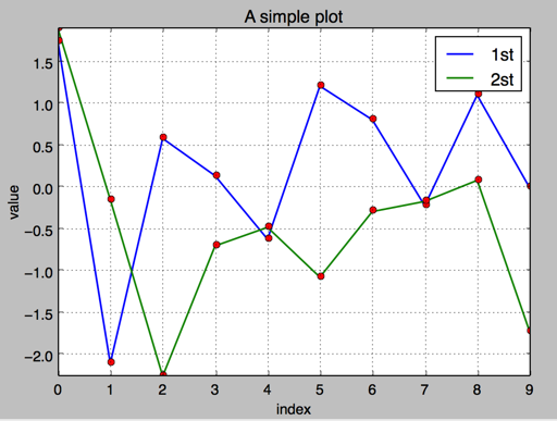
2.添加图例 plt.legend(loc = 0)
#!/etc/bin/python
#coding=utf-8
import numpy as np
import matplotlib as mpl
import matplotlib.pyplot as plt

np.random.seed(2000)
y = np.random.standard_normal((10, 2))
plt.figure(figsize=(7,5))
plt.plot(y[:,0], lw = 1.5,label = '1st')
plt.plot(y[:,1], lw = 1.5, label = '2st')
plt.plot(y, 'ro')
plt.grid(True)
plt.legend(loc = 0) #图例位置自动
plt.axis('tight')
plt.xlabel('index')
plt.ylabel('value')
plt.title('A simple plot')
plt.show()
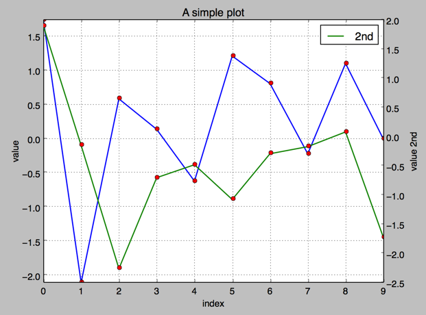
.使用2个 Y轴(左右)fig, ax1 = plt.subplots() ax2 = ax1.twinx()
#!/etc/bin/python
#coding=utf-8
import numpy as np
import matplotlib as mpl
import matplotlib.pyplot as plt

np.random.seed(2000)
y = np.random.standard_normal((10, 2))

fig, ax1 = plt.subplots() # 关键代码1 plt first data set using first (left) axis

plt.plot(y[:,0], lw = 1.5,label = '1st')

plt.plot(y[:,0], 'ro')
plt.grid(True)
plt.legend(loc = 0) #图例位置自动
plt.axis('tight')
plt.xlabel('index')
plt.ylabel('value')
plt.title('A simple plot')

ax2 = ax1.twinx()  #关键代码2  plt second data set using second(right) axis
plt.plot(y[:,1],'g', lw = 1.5, label = '2nd')
plt.plot(y[:,1], 'ro')
plt.legend(loc = 0)
plt.ylabel('value 2nd')
plt.show()
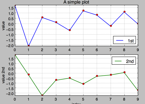
使用两个子图(上下,左右)plt.subplot(211)
通过使用 plt.subplots 函数,可以直接访问底层绘图对象,例如可以用它生成和第一个子图共享 x 轴的第二个子图.
#!/etc/bin/python
#coding=utf-8
import numpy as np
import matplotlib as mpl
import matplotlib.pyplot as plt

np.random.seed(2000)
y = np.random.standard_normal((10, 2))

plt.figure(figsize=(7,5))
plt.subplot(211)  #两行一列,第一个图
plt.plot(y[:,0], lw = 1.5,label = '1st')
plt.plot(y[:,0], 'ro')
plt.grid(True)
plt.legend(loc = 0) #图例位置自动
plt.axis('tight')
plt.ylabel('value')
plt.title('A simple plot')


plt.subplot(212) #两行一列.第二个图
plt.plot(y[:,1],'g', lw = 1.5, label = '2nd')
plt.plot(y[:,1], 'ro')
plt.grid(True)
plt.legend(loc = 0)
plt.xlabel('index')
plt.ylabel('value 2nd')
plt.axis('tight')
plt.show()