Elasticsearch简介
Elasticsearch是一个基于Apache lucene的实时分布式搜索。具有以下优点:
1、实时处理大规模数据。2、全文检索,能够做到结构化检索和聚合分析。3、分布式系统。
这些优点形成了以下的应用场景:
1、站内搜索。2、NoSQL Json文档数据库,读写性能均高于MongoDB。3、搭建日志平台用于统计、监控和分析。
Elasticsearch基本概念
- 节点(Node):物理概念,一个运行的Elasticsearch,一般是位于一台机器上的一个进程。
- 索引(Index):逻辑概念,包括配置信息mapping和倒排索引数据文件,一个索引的数据文件可能会分布于一台机器,也有可能分布于多台机器。
- 分片(Shard):为了支持更大量的数据,索引一般会按某种维度分成多个部分,每个部分就是一个分片,分片被节点(Node)管理。一个节点一般会管理多个分片,这些分片可能是属于同一份索引,也可能属于不同的索引,但是为了可靠性和可用性,同一个索引的分片尽量会分布在不同节点(Node)上。分片有两种,主分片(Primary Shard)和副本分片(Replica Shard)。
- 副本分片(Replica Shard):同一个分片(Shard)的备份数据,一个分片可能会有0个或多个副本,这些副本中的数据保证强一致或最终一致。
分片的分布图如下:

节点类型
一个Elasticsearch实例是一个节点,一组节点组成了集群。Elasticsearch集群中的节点可以配置为3种不同的角色:
-
主节点:控制Elasticsearch集群,负责集群中的操作,比如创建/删除一个索引,跟踪集群中的节点,分配分片到节点。主节点处理集群的状态并广播到其他节点,并接收其他节点的确认响应。
每个节点都可以通过设定配置文件elasticsearch.yml中的node.master属性为true(默认)成为主节点。
对于大型的生产集群来说,推荐使用一个专门的主节点来控制集群,该节点将不处理任何用户请求。主节点最好只有一个,用来控制和调配集群级的扩展。
-
数据节点(Data Node):持有数据和倒排索引。默认情况下,每个节点都可以通过设定配置文件elasticsearch.yml中的node.data属性为true(默认)成为数据节点。如果我们要使用一个专门的主节点,应将其node.data属性设置为false。
-
客户端节点(Transport Node):如果我们将node.master属性和node.data属性都设置为false,那么该节点就是一个客户端节点,扮演一个负载均衡的角色,将到来的请求路由到集群中的各个节点。
Elasticsearch集群中作为客户端接入的节点叫协调节点。协调节点会将客户端请求路由到集群中合适的分片上。对于读请求来说,协调节点每次会选择不同的分片处理请求,以实现负载均衡。
节点部署方式
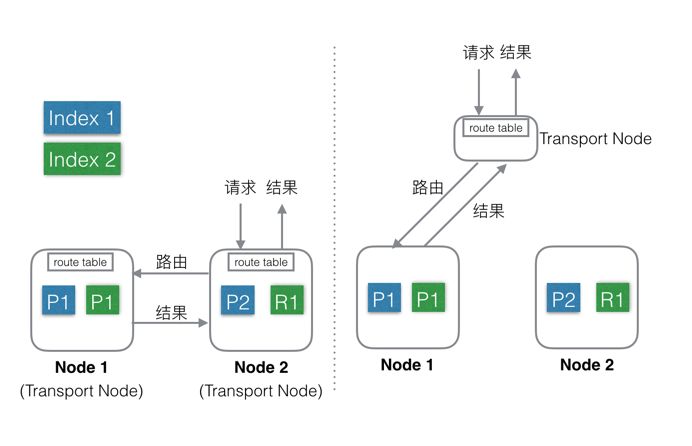
Elasticsearch支持上述两种部署方式:
第一种:混合部署(如左图),不考虑MasterNode的情况下,还有两种Node,Data Node和Transport Node,这种部署模式下,这两种不同类型Node角色都位于同一个Node中,相当于一个Node具备两种功能:Data和Transport。
当有index或者query请求的时候,请求随机(自定义)发送给任何一个Node,这台Node中会持有一个全局的路由表,通过路由表选择合适的Node,将请求发送给这些Node,然后等所有请求都返回后,合并结果,然后返回给用户。一个Node分饰两种角色。
好处就是使用极其简单,易上手,对推广系统有很大价值。最简单的场景下只需要启动一个Node,就能完成所有的功能。
缺点就是:1、多种类型的请求会相互影响,在大集群如果某一个Data Node出现热点,那么就会影响途经这个Data Node的所有其他跨Node请求。如果发生故障,故障影响面会变大很多。
2、Elasticsearch中每个Node都需要和其余的每一个Node都保持着连接。这种情况下,每个Node都需要和其他所有Node保持连接,而一个系统的连接数是有上限的,这样连接数就会限制集群规模。
3、还有就是不能支持集群的热更新。
第二种:分层部署(如右图),通过配置可以隔离开Node。设置部分Node为Transport Node,专门用来做请求转发和结果合并。其他Node可以设置为DataNode,专门用来处理数据。
缺点是上手复杂,需要提前设置好Transport的数量,且数量和Data Node、流量等相关,否则要么资源闲置,要么机器被打爆。
好处就是:1、角色相互独立,不会相互影响,一般Transport Node的流量是平均分配的,很少出现单台机器的CPU或流量被打满的情况,而DataNode由于处理数据,很容易出现单机资源被占满,比如CPU,网络,磁盘等。独立开后,DataNode如果出了故障只是影响单节点的数据处理,不会影响其他节点的请求,影响限制在最小的范围内。
2、角色独立后,只需要Transport Node连接所有的DataNode,而DataNode则不需要和其他DataNode有连接。一个集群中DataNode的数量远大于Transport Node,这样集群的规模可以更大。另外,还可以通过分组,使Transport Node只连接固定分组的DataNode,这样Elasticsearch的连接数问题就彻底解决了。
3、可以支持热更新:先一台一台的升级DataNode,升级完成后再升级Transport Node,整个过程中,可以做到让用户无感知。
Elasticsearch 数据层架构
数据存储
Elasticsearch的Index和meta,目前支持存储在本地文件系统中,同时支持niofs,mmap,simplefs,smb等不同加载方式,性能最好的是直接将索引LOCK进内存的MMap方式。默认,Elasticsearch会自动选择加载方式,另外可以自己在配置文件中配置。这里有几个细节,具体可以看官方文档。
索引和meta数据都存在本地,会带来一个问题:当某一台机器宕机或者磁盘损坏的时候,数据就丢失了。为了解决这个问题,可以使用Replica(副本)功能。
副本(Replica)
可以为每一个Index设置一个配置项:副本(Replica)数,如果设置副本数为2,那么就会有3个Shard,其中一个是Primary Shard,其余两个是Replica Shard,这三个Shard会被Master尽量调度到不同机器,甚至机架上,这三个Shard中的数据一样,提供同样的服务能力。副本(Replica)的目的有三个:
- 保证服务可用性:当设置了多个Replica的时候,如果某一个Replica不可用的时候,那么请求流量可以继续发往其他Replica,服务可以很快恢复开始服务。
- 保证数据可靠性:如果只有一个Primary,没有Replica,那么当Primary的机器磁盘损坏的时候,那么这个Node中所有Shard的数据会丢失,只能reindex了。
- 提供更大的查询能力:当Shard提供的查询能力无法满足业务需求的时候, 可以继续加N个Replica,这样查询能力就能提高N倍,轻松增加系统的并发度。
存储模型
Elasticsearch使用了Apache Lucene,后者是Doug Cutting(Apache Hadoop之父)使用Java开发的全文检索工具库,其内部使用的是被称为倒排索引的数据结构,其设计是为全文检索结果的低延迟提供服务。文档是Elasticsearch的数据单位,对文档中的词项进行分词,并创建去重词项的有序列表,将词项与其在文档中出现的位置列表关联,便形成了倒排索引。
这和一本书后面的索引非常类似,即书中包含的词汇与其出现的页码列表关联。当我们说文档被索引了,我们指的是倒排索引。我们来看下如下2个文档是如何被倒排索引的:
文档1(Doc 1): Insight Data Engineering Fellows Program
文档2(Doc 2): Insight Data Science Fellows Program

如果我们想找包含词项"insight"的文档,我们可以扫描这个(单词有序的)倒排索引,找到"insight"并返回包含改词的文档ID,示例中是Doc 1和Doc 2。
为了提高可检索性(比如希望大小写单词都返回),我们应当先分析文档再对其索引。分析包括2个部分:
- 将句子词条化为独立的单词
- 将单词规范化为标准形式
默认情况下,Elasticsearch使用标准分析器,它使用了:
- 标准分词器以单词为界来切词
- 小写词条(token)过滤器来转换单词
还有很多可用的分析器在此不列举,请参考相关文档。使用TF-IDF法计算相似度。
为了实现查询时能得到对应的结果,查询时应使用与索引时一致的分析器,对文档进行分析。
注意:标准分析器包含了停用词过滤器,但默认情况下没有启用。
剖析写操作
当我们发送索引一个新文档的请求到协调节点后,将发生如下一组操作:
-
Elasticsearch集群中的每个节点都包含了改节点上分片的元数据信息。协调节点(默认)使用文档ID参与计算,以便为路由提供合适的分片。Elasticsearch使用MurMurHash3函数对文档ID进行哈希,其结果再对分片数量取模,得到的结果即是索引文档的分片。
shard = hash(document_id) % (num_of_primary_shards)
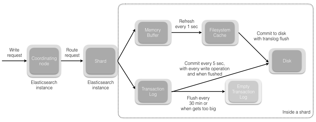
- 当分片所在的节点接收到来自协调节点的请求后,会将该请求写入translog(我们将在本系列接下来的文章中讲到),并将文档加入内存缓冲。如果请求在主分片上成功处理,该请求会并行发送到该分片的副本上。当translog被同步(fsync)到全部的主分片及其副本上后,客户端才会收到确认通知。
- 内存缓冲会被周期性刷新(默认是1秒),内容将被写到文件系统缓存的一个新段上。虽然这个段并没有被同步(fsync),但它是开放的,内容可以被搜索到。
- 每30分钟,或者当translog很大的时候,translog会被清空,文件系统缓存会被同步。这个过程在Elasticsearch中称为冲洗(flush)。在冲洗过程中,内存中的缓冲将被清除,内容被写入一个新段。段的fsync将创建一个新的提交点,并将内容刷新到磁盘。旧的translog将被删除并开始一个新的translog。
下图展示了写请求及其数据流。
更新((U)pdate)和删除((D)elete)
删除和更新也都是写操作。但是Elasticsearch中的文档是不可变的,因此不能被删除或者改动以展示其变更。那么,该如何删除和更新文档呢?
磁盘上的每个段(segment)都有一个相应的.del文件。当删除请求发送后,文档并没有真的被删除,而是在.del文件中被标记为删除。该文档依然能匹配查询,但是会在结果中被过滤掉。当段合并(我们将在本系列接下来的文章中讲到)时,在.del文件中被标记为删除的文档将不会被写入新段。
接下来我们看更新是如何工作的。在新的文档被创建时,Elasticsearch会为该文档指定一个版本号。当执行更新时,旧版本的文档在.del文件中被标记为删除,新版本的文档被索引到一个新段。旧版本的文档依然能匹配查询,但是会在结果中被过滤掉。
文档被索引或者更新后,我们就可以执行查询操作了。让我们看看在Elasticsearch中是如何处理查询请求的。
剖析读操作((R)ead)
读操作包含2部分内容:
- 查询阶段
- 提取阶段
我们来看下每个阶段是如何工作的。
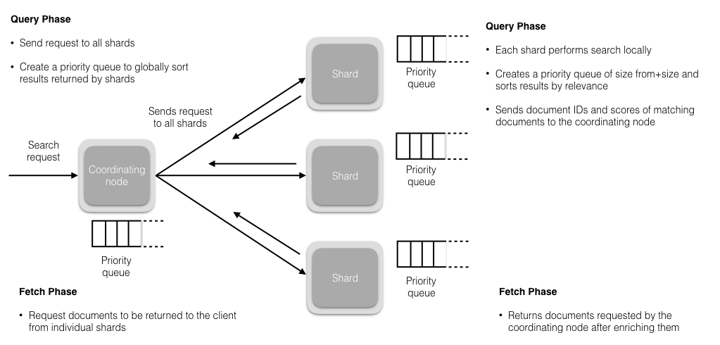
查询阶段
在这个阶段,协调节点会将查询请求路由到索引的全部分片(主分片或者其副本)上。每个分片独立执行查询,并为查询结果创建一个优先队列,以相关性得分排序(我们将在本系列的后续文章中讲到)。全部分片都将匹配文档的ID及其相关性得分返回给协调节点。协调节点创建一个优先队列并对结果进行全局排序。会有很多文档匹配结果,但是,默认情况下,每个分片只发送前10个结果给协调节点,协调节点为全部分片上的这些结果创建优先队列并返回前10个作为hit。
提取阶段
当协调节点在生成的全局有序的文档列表中,为全部结果排好序后,它将向包含原始文档的分片发起请求。全部分片填充文档信息并将其返回给协调节点。
下图展示了读请求及其数据流。
如上所述,查询结果是按相关性排序的。接下来,让我们看看相关性是如何定义的。
搜索相关性
相关性是由搜索结果中Elasticsearch打给每个文档的得分决定的。默认使用的排序算法是tf/idf(词频/逆文档频率)。词频衡量了一个词项在文档中出现的次数 (频率越高 == 相关性越高),逆文档频率衡量了词项在全部索引中出现的频率,是一个索引中文档总数的百分比(频率越高 == 相关性越低)。最后的得分是tf-idf得分与其他因子比如(短语查询中的)词项接近度、(模糊查询中的)词项相似度等的组合。
Elasticsearch three Cs(Consensus, Concurrency, Consistency)
Consensus
Consensus is one of the fundamental challenges of a distributed system. It requires all the processes/nodes in the system to agree on a given data value/status. There are a lot of consensus algorithms like Raft, Paxos, etc. which are mathematically proven to work, however, Elasticsearch has implemented its own consensus system (zen discovery) because of reasons described here by Shay Banon (Elasticsearch creator). The zen discovery module has two parts:
- Ping: The process nodes use to discover each other.
- Unicast: The module that contains a list of hostnames to control which nodes to ping.
Elasticsearch is a peer-to-peer system where all nodes communicate with each other and there is one active master which updates and controls the cluster wide state and operations. A new Elasticsearch cluster undergoes an election as part of the ping process where a node, out of all master eligible nodes, is elected as the master and other nodes join the master. The default ping_interval is 1 sec and ping_timeout is 3 sec. As nodes join, they send a join request to the master with a default join_timeout which is 20 times the ping_timeout. If the master fails, the nodes in the cluster start pinging again to start another election. This ping process also helps if a node accidentally thinks that the master has failed and discovers the master through other nodes.
For fault detection, the master node pings all the other nodes to check if they are alive and all the nodes ping the master back to report that they are alive.
If used with the default settings, Elasticsearch suffers from the problem of split-brain where in case of a network partition, a node can think that the master is dead and elect itself as a master resulting in a cluster with multiple masters. This may result in data loss and it may not be possible to merge the data correctly. This can be avoided by setting the following property to a quorum of master eligible nodes.
-
discovery.zen.minimum_master_nodes = int(# of master eligible nodes/2)+1

NOTE: For a production cluster, it is recommended to have 3 dedicated master nodes, which do not serve any client requests, out of which 1 is active at any given time.
As we have learned about consensus in Elasticsearch, let’s now see how it deals with concurrency.
Concurrency
Elasticsearch is a distributed system and supports concurrent requests. When a create/update/delete request hits the primary shard, it is sent in parallel to the replica shard(s) as well, however, it is possible that these requests arrive out of order. In such cases, Elasticsearch uses optimistic concurrency controlto make sure that the newer versions of the document are not overwritten by the older versions.
Every document indexed has a version number which is incremented with every change applied to that document. These version numbers are used to make sure that the changes are applied in order. To make sure that updates in our application don’t result in data loss, Elasticsearch’s API allows you to specify the current version number of a document to which the changes should be applied. If the version specified in the request is older than the one present in the shard, the request fails, which means that the document has been updated by another process. How failed requests are handled can be controlled at the application level. There are also other locking options available and you can read about them here.
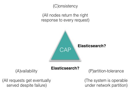
As we send concurrent requests to Elasticsearch, the next concern is — how can we make these requests consistent? Now, it is unclear to answer which side of the CAP triangle Elasticsearch falls on and this has been a debate which we are not going to settle in this post.
Consistency — Ensuring consistent writes and reads
For writes, Elasticsearch supports consistency levels, different from most other databases, to allow a preliminary check to see how many shards are available for the write to be permissible. The available options are quorum, one and all. By default it is set to quorum and that means that a write operation will be permitted only if a majority of the shards are available. With a majority of the shards available, it may still happen that the writes to a replica fail for some reason and in that case, the replica is said to be faulty and the shard would be rebuilt on a different node.
For reads, new documents are not available for search until after the refresh interval. To make sure that the search request returns results from the latest version of the document, replication can be set to sync (default) which returns the write request after the operation has been completed on both primary and replica shards. In this case, search request from any shard will return results from the latest version of the document. Even if your application requires replication=async for higher indexing rate, there is a _preference parameter which can be set to primary for search requests. That way, the primary shard is queried for search requests and it ensures that the results will be from the latest version of the document.
As we understand how Elasticsearch deals with consensus, concurrency and consistency, let’s review some of the important concepts internal to a shard that result in certain characteristics of Elasticsearch as a distributed search engine.
Translog
The concept of a write ahead log (WAL) or a transaction log (translog) has been around in the database world since the development of relational databases. A translog ensures data integrity in the event of failure with the underlying principle that the intended changes must be logged and committed before the actual changes to the data are committed to the disk.
When new documents are indexed or old ones are updated, the Lucene index changes and these changes will be committed to the disk for persistence. It is a very expensive operation to be performed after every write request and hence, it is performed in a way to persist multiple changes to the disk at once. As we described in a previous blog, flush operation (Lucene commit) is performed by default every 30 min or when the translog gets too big (default is 512MB). In such a scenario, there is a possibility to lose all the changes between two Lucene commits. To avoid this issue, Elasticsearch uses a translog. All the index/delete/update operations are written to the translog and the translog is fsync’ed after every index/delete/update operation (or every 5 sec by default) to make sure the changes are persistent. The client receives acknowledgement for writes after the translog is fsync’ed on both primary and replica shards.
In case of a hardware failure between two Lucene commits or a restart, the translog is replayed to recover from any lost changes before the last Lucene commit and all the changes are applied to the index.
NOTE: It is recommended to explicitly flush the translog before restarting Elasticsearch instances, as the startup will be faster because the translog to be replayed will be empty. POST /_all/_flush command can be used to flush all indices in the cluster.
With the translog flush operation, the segments in the filesystem cache are committed to the disk to make changes in the index persistent. Let’s now see what Lucene segments are.
Lucene Segments
A Lucene index is made up of multiple segments and a segment is a fully functional inverted index in itself. Segments are immutable which allows Lucene to add new documents to the index incrementally without rebuilding the index from scratch. For every search request, all the segments in an index are searched, and each segment consumes CPU cycles, file handles and memory. This means that the higher the number of segments, the lower the search performance will be.
To get around this problem, Elasticsearch merges small segments together into a bigger segment (as shown in the figure below), commits the new merged segment to the disk and deletes the old smaller segments.
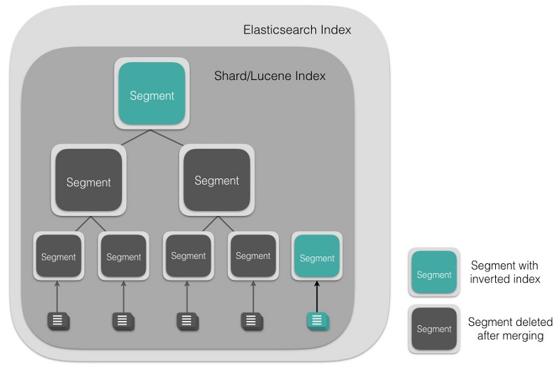
This automatically happens in the background without interrupting indexing or searching. Since segment merging can use up resources and affect search performance, Elasticsearch throttles the merging process to have enough resources available for search.
Anatomy of an Elasticsearch Cluster: Part II
Near real-time search
While changes in Elasticsearch are not visible right away, it does offer a near real-time search engine. As mentioned in a previous post, committing Lucene changes to disk is an expensive operation. To avoid committing changes to disk while still make documents available for search, there is a filesystem cache sitting in between the memory buffer and the disk. The memory buffer is refreshed every second (by default) and a new segment, with the inverted index, is created in the filesystem cache. This segment is opened and made available for search.
A filesystem cache can have file handles and files can be opened, read and closed, however, it lives in memory. Since, the refresh interval is 1 sec by default, the changes are not visible right away and hence it is near real-time. Since, the translog is a persistent record of changes not persisted to the disk, it also helps with the near real-time aspect for CRUD operations. For every request, the translog is searched for any recent changes before looking into relevant segments and hence, the client has access to all the changes in near real-time.
You can explicitly refresh the index after every Create/Update/Delete operation to make the changes visible right away but it is not recommended as it affects the search performance due to too many small segments being created. For a search request, all Lucene segments in a given shard of an Elasticsearch index are searched, however, fetching all matching documents or documents deep in the resulting pages is dangerous for your Elasticsearch cluster. Let’s see why that is.
Why deep pagination in distributed search can be dangerous?
When you make a search request in Elasticsearch which has a lot of matching documents, by default, the first page returned consists of the top 10 results. The search API has from and size parameters to specify how deep the results should be for all the documents that match the search. For instance, if you want to see the documents with ranks 50 to 60 that match the search, then from=50 and size=10. When each shard receives the search request, it creates a priority queue of size from+size to satisfy the search result itself and then returns the results to the coordinating node.
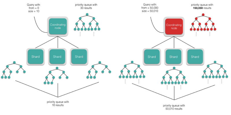
If you want to see results ranked from 50,000 to 50,010, then each shard will create a priority queue with 50,010 results each, and the coordinating node will have to sort number of shards * 50,010 results in memory. This level of pagination may or may not be possible depending upon the hardware resources you have but it suffices to say that you should be very careful with deep pagination as it can easily crash your cluster.
It is possible to get all the documents that match the result using the scroll APIwhich acts more like a cursor in relational databases. Sorting is disabled with the scroll API and each shard keeps sending results as long as it has documents that match the search.
Sorting scored results is expensive if a large number of documents are to be fetched. And since Elasticsearch is a distributed system, calculating the search relevance score for a document is very expensive. Let’s now see one of the many trade-offs made to calculate search relevance.
Trade-offs in calculating search relevance
Elasticsearch uses tf-idf for search relevance and because of its distributed nature, calculating a global idf (inverse document frequency) is very expensive. Instead, every shard calculates a local idf to assign a relevance score to the resulting documents and returns the result for only the documents on that shard. Similarly, all the shards return the resulting documents with relevant scores calculated using local idf and the coordinating node sorts all the results to return the top ones. This is fine in most cases, unless your index is skewed in terms of keywords or there is not enough data on a single shard to represent the global distribution.
For instance, if you are searching for the word “insight” and a majority of the documents containing the term “insight” reside on one shard, then the documents that match the query won’t be fairly ranked on each shard as the local idf values will vary greatly and the search results might not be very relevant. Similarly, if there is not enough data, then the local idf values may vary greatly for some searches and the results might not be as relevant as expected. In real-world scenarios with enough data, the local idf values tend to even out and search results are relevant as the documents are fairly scored.
There are a couple of ways to get around the local idf score but they are not really recommended for production systems.
- One way is that you can have just one shard for the index and then the local idf is the global idf, but this doesn’t leave room for parallelism/scaling and isn’t practical for huge indices.
- Another way is to use a parameter dfs_query_then_search (dfs = distributed frequency search) with the search request, which calculates local idf for all shards first, then combines these local idf values to calculate a global idf for the entire index and then returns the results with the relevance score calculated using the global idf. This isn’t recommended in production and having enough data would ensure that the term frequencies are well distributed.
In the last few posts, we reviewed some of the fundamental principles of Elasticsearch which are important to understand in order to get started. In a follow up post, I will be going through indexing data in Elasticsearch using Apache Spark.
Anatomy of an Elasticsearch Cluster: Part III