课程五(Sequence Models)，第三周（Sequence models & Attention mechanism） —— 2.Programming assignments：Trigger word detection

Expected OutputTrigger Word Detection

Welcome to the final programming assignment of this specialization!

In this week's videos, you learned about applying deep learning to speech recognition. In this assignment, you will construct a speech dataset and implement an algorithm for trigger word detection (sometimes also called keyword detection, or wakeword detection). Trigger word detection is the technology that allows devices like Amazon Alexa, Google Home, Apple Siri, and Baidu DuerOS to wake up upon hearing a certain word.

For this exercise, our trigger word will be "Activate." Every time it hears you say "activate," it will make a "chiming" sound. By the end of this assignment, you will be able to record a clip of yourself talking, and have the algorithm trigger a chime when it detects you saying "activate."

After completing this assignment, perhaps you can also extend it to run on your laptop so that every time you say "activate" it starts up your favorite app, or turns on a network connected lamp in your house, or triggers some other event。

In this assignment you will learn to:

Structure a speech recognition project
Synthesize and process audio recordings to create train/dev datasets
Train a trigger word detection model and make predictions

【中文翻译】

触发字检测

欢迎来到这个专业化的最终编程任务!

在本周的视频中, 您了解了如何将深度学习应用于语音识别。在这个任务中, 您将构造一个语音数据集并实现触发字检测 (有时也称为关键字检测或 wakeword 检测) 的算法。触发字检测是一种技术, 它允许亚马逊 Alexa、谷歌主页、苹果 Siri 和百度 DuerOS 等设备在听到某个单词时醒来。

对于本练习, 我们的触发器词是 "Activate". 每次听到您说 "Activate" 时, 都会发出 "chiming " 声音。完成此任务后, 您将能够录制自己说话的剪辑, 并且在检测到您说 "activate" 时, 该算法会触发一个chime。

完成此任务后, 您可能还可以将其扩展到laptop上运行, 以便每次您说 "activate ", 就会启动您喜欢的应用程序, 或打开您的房子中的链接了网络的灯, 或触发其他事件。

在这个作业中, 您将学习:

构造语音识别项目
合成和处理录音以创建训练/开发数据集
训练触发字检测模型并进行预测

Lets get started! Run the following cell to load the package you are going to use.

【code】

import numpy as np
from pydub import AudioSegment
import random
import sys
import io
import os
import glob
import IPython
from td_utils import *
%matplotlib inline

1 - Data synthesis: Creating a speech dataset

Let's start by building a dataset for your trigger word detection algorithm. A speech dataset should ideally be as close as possible to the application you will want to run it on. In this case, you'd like to detect the word "activate" in working environments (library, home, offices, open-spaces ...). You thus need to create recordings with a mix of positive words ("activate") and negative words (random words other than activate) on different background sounds. Let's see how you can create such a dataset.

【中文翻译】

让我们首先构建一个数据集, 用于触发词检测算法。语音数据集最好尽可能靠近要运行它的应用程序。在这种情况下, 您希望在工作环境 (图书馆、家里、办公室、开放空间...) 中检测单词 "激活 "。因此, 您需要在不同的背景声音中创建带有 positive words ( "activate ") 和negative words (除了激活以外的随机单词) 的混合的录制。让我们看看如何创建这样的数据集。

1.1 - Listening to the data

One of your friends is helping you out on this project, and they've gone to libraries, cafes, restaurants, homes and offices all around the region to record background noises, as well as snippets of audio of people saying positive/negative words. This dataset includes people speaking in a variety of accents.

In the raw_data directory, you can find a subset of the raw audio files of the positive words, negative words, and background noise. You will use these audio files to synthesize a dataset to train the model. The "activate" directory contains positive examples of people saying the word "activate". The "negatives" directory contains negative examples of people saying random words other than "activate". There is one word per audio recording. The "backgrounds" directory contains 10 second clips of background noise in different environments.

【中文翻译】

你的一个朋友正在帮助你这个项目, 他们已经去图书馆, 咖啡馆, 餐馆, 家庭和办公室各地的地区, 以记录背景噪音, 以及包含人说积极/否定词的音频片段。这个数据集包括用各种口音说话的人。

在 raw_data 目录中, 您可以找到positive words、negative words和背景噪音的原始音频文件的子集。您将使用这些音频文件合成数据集来训练模型。 "activate " 目录包含一些人说 "activate " 这个词的正面例子。"negatives " 目录中包含一些负面的例子, 说明其他人说的是随机单词。每个录音都有一个字。 "backgrounds " 目录在不同环境中包含10秒的背景噪音片段。

Run the cells below to listen to some examples.

【code】

IPython.display.Audio("./raw_data/activates/1.wav")

【result】

【注】原网页是音频，发出activate的声音。这里是截图。

【code】

IPython.display.Audio("./raw_data/negatives/4.wav")

【result】

【注】原网页是音频。这里是截图。

【code】

IPython.display.Audio("./raw_data/backgrounds/1.wav")

【result】

【注】原网页是音频。这里是截图。　　

You will use these three type of recordings (positives/negatives/backgrounds) to create a labelled dataset.　　

1.2 - From audio recordings to spectrograms

What really is an audio recording? A microphone records little variations in air pressure over time, and it is these little variations in air pressure that your ear also perceives as sound. You can think of an audio recording is a long list of numbers measuring the little air pressure changes detected by the microphone. We will use audio sampled at 44100 Hz (or 44100 Hertz). This means the microphone gives us 44100 numbers per second. Thus, a 10 second audio clip is represented by 441000 numbers (=

It is quite difficult to figure out from this "raw" representation of audio whether the word "activate" was said. In order to help your sequence model more easily learn to detect triggerwords, we will compute a spectrogram of the audio. The spectrogram tells us how much different frequencies are present in an audio clip at a moment in time.

(If you've ever taken an advanced class on signal processing or on Fourier transforms, a spectrogram is computed by sliding a window over the raw audio signal, and calculates the most active frequencies in each window using a Fourier transform. If you don't understand the previous sentence, don't worry about it.)

【中文翻译】

1.2-从录音到图谱
什么是录音？麦克风记录了随着时间的推移, 气压的微小变化, 这是空气压力的小变化, 你的耳朵觉察到声音。你可以认为录音是一长串的数字, 测量麦克风检测到的小气压变化。我们将使用音频采样，在44100赫兹。这意味着麦克风每秒给我们44100个数字。因此, 10 秒的音频剪辑由441000个数字 (= 10×4410010) 表示。

从这个 "原始 " 的音频中,判断"activate " 这个词是否说了是相当困难的。为了帮助您的序列模型更容易地学会检测 triggerwords, 我们将计算音频的频谱图。频谱图告诉我们在某一时刻音频剪辑中有多少不同的频率。

(如果您曾经上过信号处理或傅立叶变换这类的课, 则会知道，通过将窗口滑动在原始音频信号滑动来计算频谱图, 并使用傅立叶变换计算每个窗口中最活跃的频率。如果你不理解前一句话, 不要担心。）

Lets see an example.

【code】

IPython.display.Audio("audio_examples/example_train.wav")

【result】

【注】原网页是音频。这里是截图。

【code】

x = graph_spectrogram("audio_examples/example_train.wav")

【result】

The graph above represents how active each frequency is (y axis) over a number of time-steps (x axis).

【中文翻译】

图 1: 音频记录的频谱图谱, 其中的颜色显示不同频率 (响亮) 在不同时间点的音频中存在的程度。绿色正方形意味某一频率是更加活跃或更多存，在在音频片段 (更大);蓝色方块表示频率较少。

The dimension of the output spectrogram depends upon the hyperparameters of the spectrogram software and the length of the input. In this notebook, we will be working with 10 second audio clips as the "standard length" for our training examples. The number of timesteps of the spectrogram will be 5511. You'll see later that the spectrogram will be the input

输出频谱图的维度取决于频谱图软件的 hyperparameters 和输入的长度。在本笔记本中, 我们将使用10秒的音频剪辑作为我们的训练样本的 "标准长度 "。频谱图的 timesteps 数将为5511。稍后您将看到频谱图将作为x输入到网络中, 因此 T_x=5511。

【code】

_, data = wavfile.read("audio_examples/example_train.wav")
print("Time steps in audio recording before spectrogram", data[:,0].shape)
print("Time steps in input after spectrogram", x.shape)

【result】

Time steps in audio recording before spectrogram (441000,)
Time steps in input after spectrogram (101, 5511)

Now, you can define:　　

Tx = 5511 # The number of time steps input to the model from the spectrogram                  从频谱图向模型输入的时间步长数
n_freq = 101 # Number of frequencies input to the model at each time step of the spectrogram  在频谱图的每个时间步骤中向模型输入的频率数

Note that even with 10 seconds being our default training example length, 10 seconds of time can be discretized to different numbers of value. You've seen 441000 (raw audio) and 5511 (spectrogram). In the former case, each step represents

For the 10sec of audio, the key values you will see in this assignment are:

Note that each of these representations correspond to exactly 10 seconds of time. It's just that they are discretizing them to different degrees. All of these are hyperparameters and can be changed (except the 441000, which is a function of the microphone). We have chosen values that are within the standard ranges uses for speech systems.

Consider the

Consider also the 10000 number above. This corresponds to discretizing the 10sec clip into 10/10000 = 0.001 second itervals. 0.001 seconds is also called 1 millisecond, or 1ms. So when we say we are discretizing according to 1ms intervals, it means we are using 10,000 steps.

【中文翻译】

请注意, 即使10秒是我们的默认训练示例长度, 10 秒的时间可以被离散到不同的值数。您已经看到 441000 (原始音频) 和 5511 (频谱图)。在前一种情况下, 每个步骤表示10秒/441000≈0.000023 秒钟。在第二种情况下, 每个步骤代表 10/5511≈0.0018 秒。

对于10sec 的音频, 您将在该作业中看到的关键值是:

441000 (原始音频)
5511 = T_x (频谱图输出和输入到神经网络的维度)。
10000 (由 pydub 模块合成音频)
1375 = T_y (您要构建的 GRU 的输出中的步骤数)。

请注意, 每个表示形式对应的时间正好为10秒。只是他们离散不同的程度。所有这些都是 hyperparameters , 可以改变 (除了 441000, 这是麦克风的功能)。我们选择了在语音系统的标准范围内使用的值。

请考虑上面的 T_y=1375 。这意味着, 对于模型的输出, 我们将10s 离散为1375个时间间隔 (每个长度 10/1375≈0.0072s), 并尝试预测每个间隔是否有人最近完成了 "activate"。

还要考虑上面的10000个数字。这对应于将10s 离散为10000个时间间隔 (每个长度0/10000 = 0.001s), 0.001 秒也称为1毫秒或1ms。所以, 当我们说, 我们根据1ms 的时间间隔离散, 这意味着我们使用10,000步骤。

【code】

Ty = 1375 # The number of time steps in the output of our model 模型输出中的时间步长数

1.3 - Generating a single training example

Because speech data is hard to acquire and label, you will synthesize your training data using the audio clips of activates, negatives, and backgrounds. It is quite slow to record lots of 10 second audio clips with random "activates" in it. Instead, it is easier to record lots of positives and negative words, and record background noise separately (or download background noise from free online sources).

To synthesize a single training example, you will:

Pick a random 10 second background audio clip
Randomly insert 0-4 audio clips of "activate" into this 10sec clip
Randomly insert 0-2 audio clips of negative words into this 10sec clip

Because you had synthesized the word "activate" into the background clip, you know exactly when in the 10sec clip the "activate" makes its appearance. You'll see later that this makes it easier to generate the labels

You will use the pydub package to manipulate audio. Pydub converts raw audio files into lists of Pydub data structures (it is not important to know the details here). Pydub uses 1ms as the discretization interval (1ms is 1 millisecond = 1/1000 seconds) which is why a 10sec clip is always represented using 10,000 steps.

【中文翻译】

由于语音数据难以获取和标记, 您将使用activates, negatives, and backgrounds的音频剪辑来合成训练数据。在其中随机 "activates " ,录制大量10秒的音频剪辑是相当缓慢的。相反, 记录大量的 positive 和 negative的单词, 并单独记录背景噪音 (或从免费的在线来源下载背景噪音)是更容易的。

要合成一个训练样本, 您将:

选择随机10秒背景音频剪辑
随机插入0-4 音频剪辑 "activate" 到这个10sec 剪辑
在10sec 剪辑中随机插入0-2 个negative 单词的音频剪辑

因为您已将单词 "activate " 合成到背景剪辑中, 所以您确切知道在10sec 剪辑中 "activate " 的出现。稍后您将看到, 这使得生成标签 y^⟨t⟩也更容易。

您将使用 pydub 包来操作音频。Pydub 将原始音频文件转换为 Pydub 数据结构列表 (在此处了解详细信息，但并不重要)。Pydub 使用1ms 作为离散化间隔 (1ms 是1毫秒 = 1/1000 秒), 这就是为什么10sec 剪辑总是使用1万个步骤表示的原因。

【code】

# Load audio segments using pydub 
activates, negatives, backgrounds = load_raw_audio()

print("background len: " + str(len(backgrounds[0])))    # Should be 10,000, since it is a 10 sec clip
print("activate[0] len: " + str(len(activates[0])))     # Maybe around 1000, since an "activate" audio clip is usually around 1 sec (but varies a lot)
print("activate[1] len: " + str(len(activates[1])))     # Different "activate" clips can have different lengths

【result】

background len: 10000
activate[0] len: 916
activate[1] len: 1579

Overlaying positive/negative words on the background:

Given a 10sec background clip and a short audio clip (positive or negative word), you need to be able to "add" or "insert" the word's short audio clip onto the background. To ensure audio segments inserted onto the background do not overlap, you will keep track of the times of previously inserted audio clips. You will be inserting multiple clips of positive/negative words onto the background, and you don't want to insert an "activate" or a random word somewhere that overlaps with another clip you had previously added.

For clarity, when you insert a 1sec "activate" onto a 10sec clip of cafe noise, you end up with a 10sec clip that sounds like someone sayng "activate" in a cafe, with "activate" superimposed on the background cafe noise. You do not end up with an 11 sec clip. You'll see later how pydub allows you to do this.

【中文翻译】　　

在background上叠加positive/negative词:

给定10sec 背景剪辑和短音频剪辑 (positive or negative 单词), 您需要能够在背景上 "添加 " 或将单词的短音频剪辑插入。要确保插入到背景上的音频段不重叠, 您将跟踪以前插入的音频剪辑的时间。您将在背景上插入多个positive or negative 单词剪辑, 并且不希望在与以前添加的其他剪辑重叠的地方插入 "activate " 或随机单词。

为清楚起见, 当您插入 1sec "activate " 到10sec 剪辑的咖啡馆噪音, 你结束了一个10sec 剪辑, 听起来像有人说 "激活 " 在咖啡馆, 。你不会得到一个11秒的剪辑。稍后您将看到 pydub 如何允许您这样做。

Creating the labels at the same time you overlay:

Recall also that the labels

When you insert or overlay an "activate" clip, you will also update labels for

This is another reason for synthesizing the training data: It's relatively straightforward to generate these labels

【中文翻译】

在合成的同时创建标签:

还记得标签 y^⟨t⟩代表是否有人刚刚说 "activate". 给定一个背景剪辑, 我们可以对所有 t 初始化 y^⟨t⟩=0, 因为剪辑不包含任何 "激活"。

当您插入或覆盖 "activate" 剪辑时, 您还将更新 y^⟨t⟩的标签, 以便输出的50步现在具有目标标签1。您将训练一个 GRU, 以检测何时有人已完成说 "activate "。例如, 假设合成 "activate " 剪辑结束于10sec 音频中的5sec 标记,---恰好位于剪辑的一半处。还记得T_y=1375, 因此 timestep 687 = int (1375 * 0.5) 对应于音频的第5sec 。所以, 你会设置 y^⟨688⟩=1。此外, 如果 GRU 在这时刻的之后的短时间内的任何位置检测 "activate ",我们是很高兴的。那么我们实际上将连续50个标签 y^⟨t⟩的值设置为1。具体地说, 我们有 y⟨688⟩=y⟨689⟩=⋯=y⟨737⟩=1。

这是合成训练数据的另一个原因: 按照上面的描述, 生成这些标签 y^⟨t⟩相对简单。相比之下, 如果在麦克风上录制了10sec 音频, 那么一个人听它, 并在 "activate " 完成时手动标记是相当耗时的。

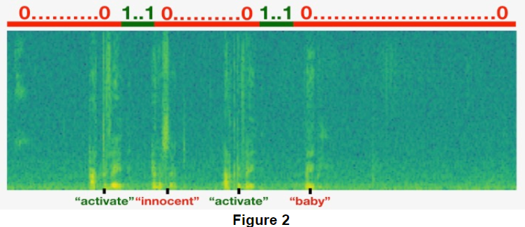
Here's a figure illustrating the labels

To implement the training set synthesis process, you will use the following helper functions. All of these function will use a 1ms discretization interval, so the 10sec of audio is alwsys discretized into 10,000 steps.

get_random_time_segment(segment_ms) gets a random time segment in our background audio
is_overlapping(segment_time, existing_segments) checks if a time segment overlaps with existing segments
insert_audio_clip(background, audio_clip, existing_times) inserts an audio segment at a random time in our background audio using get_random_time_segment and is_overlapping
insert_ones(y, segment_end_ms) inserts 1's into our label vector y after the word "activate"

The function get_random_time_segment(segment_ms) returns a random time segment onto which we can insert an audio clip of duration segment_ms. Read through the code to make sure you understand what it is doing.

【中文翻译】

这里有一个图, 说明标签 y^⟨t⟩, 对于一个剪辑, 我们已经插入 "activate", "innocent", ”activate", "baby." 。请注意, positive 标签 " 1 "只与positive的单词关联。

要实训练集的合成过程, 您将使用以下帮助函数。所有这些函数都将使用1ms 离散化间隔, 所以10sec 的音频总是离散为10000步。

get_random_time_segment (segment_ms) 在我们的背景音频中获取随机时间段
is_overlapping (segment_time、existing_segments) 检查时间段是否与现有段重叠
insert_audio_clip（ background, audio_clip, existing_times) 在我们的背景音频中使用 get_random_time_segment 和 is_overlapping 在随机时间插入音频段
insert_ones (y, segment_end_ms) 在检查到字 "activate "后，插入1到我们的标签向量 y 中。

函数 get_random_time_segment (segment_ms) 返回一个随机时间段, 我们可以在上面插入一个持续时间 segment_ms 的音频剪辑. 通读代码以确保您了解它正在做什么。

【code】

def get_random_time_segment(segment_ms):
    """
    Gets a random time segment of duration segment_ms in a 10,000 ms audio clip.
    
    Arguments:
    segment_ms -- the duration of the audio clip in ms ("ms" stands for "milliseconds")
    
    Returns:
    segment_time -- a tuple of (segment_start, segment_end) in ms
    """
    
    segment_start = np.random.randint(low=0, high=10000-segment_ms)   # Make sure segment doesn't run past the 10sec background 
    segment_end = segment_start + segment_ms - 1
    
    return (segment_start, segment_end)

Next, suppose you have inserted audio clips at segments (1000,1800) and (3400,4500). I.e., the first segment starts at step 1000, and ends at step 1800. Now, if we are considering inserting a new audio clip at (3000,3600) does this overlap with one of the previously inserted segments? In this case, (3000,3600) and (3400,4500) overlap, so we should decide against inserting a clip here.

For the purpose of this function, define (100,200) and (200,250) to be overlapping, since they overlap at timestep 200. However, (100,199) and (200,250) are non-overlapping.

【中文翻译】　　

接下来, 假设您已经在段 (1000，1800) 和 (3400，4500) 中插入了音频剪辑。即, 第一段从步骤1000开始, 在步骤1800结束。现在, 如果我们正在考虑在 (3000，3600) 中插入一个新的音频剪辑, 这与以前插入的片段有重叠吗？在这种情况下, (3000，3600) 和 (3400，4500) 重叠, 所以我们应该决定不在此插入剪辑。

为了这个函数的目的, 定义 (100，200) 和 (200，250) 重叠, 因为它们在 timestep 200 重叠。然而, (100，199) 和 (200，250) 是不重叠的。

Exercise: Implement is_overlapping(segment_time, existing_segments) to check if a new time segment overlaps with any of the previous segments. You will need to carry out 2 steps:

Create a "False" flag, that you will later set to "True" if you find that there is an overlap.
Loop over the previous_segments' start and end times. Compare these times to the segment's start and end times. If there is an overlap, set the flag defined in (1) as True. You can use:
```
for ....:
     if ... <= ... and ... >= ...:
         ...
```
Hint: There is overlap if the segment starts before the previous segment ends, and the segment ends after the previous segment starts.

【中文翻译】

练习: 实现 is_overlapping (segment_time、existing_segments) 检查新的时间段是否与前面的任何段重叠。您将需要执行2步骤:

创建一个 "False " 标志, 如果发现有重叠, 您以后将设置为 "True "。
在 previous_segments 的开始和结束时间循环。将这些时间与段的开始和结束时间进行比较。如果存在重叠, 请将 (1) 中定义的标志设置为 True。您可以使用:

    for ....:
          if ... <= ... and ... >= ...:
             ...

提示: 如果段在上一个段结束之前开始, 并且段在上一段开始后结束, 则会有重叠。

【code】

# GRADED FUNCTION: is_overlapping

def is_overlapping(segment_time, previous_segments):
    """
    Checks if the time of a segment overlaps with the times of existing segments.
    
    Arguments:
    segment_time -- a tuple of (segment_start, segment_end) for the new segment
    previous_segments -- a list of tuples of (segment_start, segment_end) for the existing segments
    
    Returns:
    True if the time segment overlaps with any of the existing segments, False otherwise
    """
    
    segment_start, segment_end = segment_time
    
    ### START CODE HERE ### (≈ 4 line)
    # Step 1: Initialize overlap as a "False" flag. (≈ 1 line)
    overlap = False
    
    # Step 2: loop over the previous_segments start and end times.
    # Compare start/end times and set the flag to True if there is an overlap (≈ 3 lines)
    for previous_start, previous_end in previous_segments:
        if segment_start <= previous_end and segment_end >= previous_start:
            overlap = True
    ### END CODE HERE ###

    return overlap

overlap1 = is_overlapping((950, 1430), [(2000, 2550), (260, 949)])
overlap2 = is_overlapping((2305, 2950), [(824, 1532), (1900, 2305), (3424, 3656)])
print("Overlap 1 = ", overlap1)
print("Overlap 2 = ", overlap2)

【result】

Overlap 1 =  False
Overlap 2 =  True

【Expected Output】

Overlap 1	False
Overlap 2	True

Now, lets use the previous helper functions to insert a new audio clip onto the 10sec background at a random time, but making sure that any newly inserted segment doesn't overlap with the previous segments.

Exercise: Implement insert_audio_clip() to overlay an audio clip onto the background 10sec clip. You will need to carry out 4 steps:

Get a random time segment of the right duration in ms.
Make sure that the time segment does not overlap with any of the previous time segments. If it is overlapping, then go back to step 1 and pick a new time segment.
Add the new time segment to the list of existing time segments, so as to keep track of all the segments you've inserted.
Overlay the audio clip over the background using pydub. We have implemented this for you.

【中文翻译】　　

现在, 让我们使用以前的帮助函数, 在随机时间将新的音频剪辑插入到10sec 背景上, 但要确保任何新插入的段不会与前面的段重叠。

练习: 实现 insert_audio_clip () 将音频剪辑覆盖到背景10sec 剪辑上。您将需要执行4步骤:

在 ms 级别，获取适当时间的随机时间段。
请确保时间段与以前的任何时间段不重叠。如果它是重叠的, 则返回步骤1并选取一个新的时间段。
将新的时间段添加到现有时间段的列表中, 以便跟踪已插入的所有段。
使用 pydub 将音频剪辑覆盖在背景上。我们已经为您实施了此项措施。

【code】

# GRADED FUNCTION: insert_audio_clip

def insert_audio_clip(background, audio_clip, previous_segments):
    """
    Insert a new audio segment over the background noise at a random time step, ensuring that the 
    audio segment does not overlap with existing segments. 在随机时间步骤中, 在背景噪音上插入新的音频段, 以确保音频段不与现有段重叠。
    
    Arguments:
    background -- a 10 second background audio recording.  
    audio_clip -- the audio clip to be inserted/overlaid. 
    previous_segments -- times where audio segments have already been placed  音频段已放置的时间
    
    Returns:
    new_background -- the updated background audio
    """
    
    # Get the duration of the audio clip in ms
    segment_ms = len(audio_clip)
    
    ### START CODE HERE ### 
    # Step 1: Use one of the helper functions to pick a random time segment onto which to insert 
    # the new audio clip. (≈ 1 line)
    segment_time = get_random_time_segment(segment_ms)
    
    # Step 2: Check if the new segment_time overlaps with one of the previous_segments. If so, keep 
    # picking new segment_time at random until it doesn't overlap. (≈ 2 lines)
    while is_overlapping(segment_time, previous_segments):
        segment_time = get_random_time_segment(segment_ms)

    # Step 3: Add the new segment_time to the list of previous_segments (≈ 1 line)
    previous_segments.append(segment_time)
    ### END CODE HERE ###
    
    # Step 4: Superpose audio segment and background 叠加音频段和背景
    new_background = background.overlay(audio_clip, position = segment_time[0])
    
    return new_background, segment_time

np.random.seed(5)
audio_clip, segment_time = insert_audio_clip(backgrounds[0], activates[0], [(3790, 4400)])
audio_clip.export("insert_test.wav", format="wav")
print("Segment Time: ", segment_time)
IPython.display.Audio("insert_test.wav")

【result】

Segment Time:  (2254, 3169)

【注】原文是音频，在背景声音中插入了“activate”音频。此处是图片。

【Expected Output】

Segment Time	(2254, 3169)

【code】

# Expected audio
IPython.display.Audio("audio_examples/insert_reference.wav")

【result】

【注】原文是音频，在背景声音中插入了“activate”音频。此处是图片。　

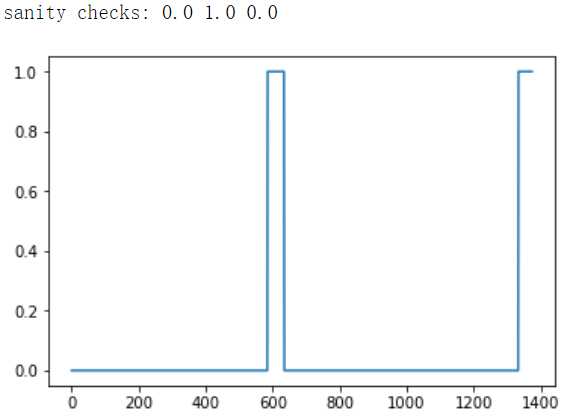
Finally, implement code to update the labels

If the "activate" ended at time step

Exercise: Implement insert_ones(). You can use a for loop. (If you are an expert in python's slice operations, feel free also to use slicing to vectorize this.) If a segment ends at segment_end_ms (using a 10000 step discretization), to convert it to the indexing for the outputs

    segment_end_y = int(segment_end_ms * Ty / 10000.0)

【中文翻译】　　

最后, 实现代码,来更新标签 y^⟨t⟩, 假设您刚刚插入了 "activate. " 在下面的代码中, y 是一个 (1，1375) 维向量, 因为 T_y=1375。

如果 "activate " 在时间步骤 t 结束, 则设置 y^⟨t+1⟩=1，以及多达49个附加的连续值也设置为1。但是, 请确保不会从数组的末尾运行, 并尝试更新 y [0] [1375], 因为有效索引是 y [0] [0] 通过 y [0] [1374], 因为 T_y=1375。所以, 如果 "activate " 结束在步骤 1370, 你会得到只有 y [0] [1371] = y [0] [1372] = y [0] [1373] = y [0] [1374] = 1

练习: 实施 insert_ones ()。可以使用 for 循环。(如果您是 python 切片操作的专家, 也可以随意使用切片量化)。如果某个段在 segment_end_ms (使用10000步离散化) 结束, 将其转换为 y (使用1375步离散化) 的输出的索引, 我们将使用此公式:

  segment_end_y = int(segment_end_ms * Ty / 10000.0)

【code】

# GRADED FUNCTION: insert_ones

def insert_ones(y, segment_end_ms):
    """
    Update the label vector y. The labels of the 50 output steps strictly after the end of the segment 
    should be set to 1. By strictly we mean that the label of segment_end_y should be 0 while, the
    50 following labels should be ones.
    更新标签向量 y。50输出步骤的标签在段结束后严格设置为1。严格来说, 我们的意思是 segment_end_y 的标签应该是 0, 而
    50 个接下来的标签应该是1。
    
    Arguments:
    y -- numpy array of shape (1, Ty), the labels of the training example
    segment_end_ms -- the end time of the segment in ms
    
    Returns:
    y -- updated labels
    """
    
    # duration of the background (in terms of spectrogram time-steps)
    segment_end_y = int(segment_end_ms * Ty / 10000.0)
    
    # Add 1 to the correct index in the background label (y)
    ### START CODE HERE ### (≈ 3 lines)
    for i in range(segment_end_y + 1, segment_end_y + 51):
        if i < Ty:
            y[0,i] =1
    ### END CODE HERE ###
    
    return y

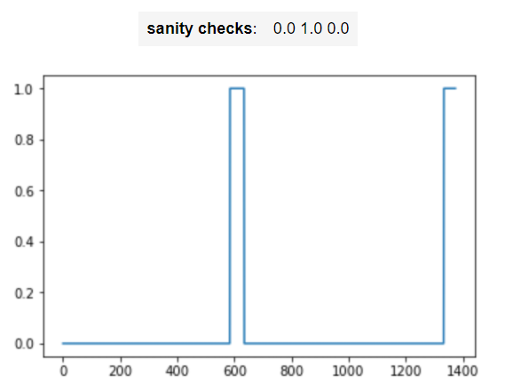
arr1 = insert_ones(np.zeros((1, Ty)), 9700)
plt.plot(insert_ones(arr1, 4251)[0,:])
print("sanity checks:", arr1[0][1333], arr1[0][634], arr1[0][635])

【result】

【Expected Output】　　

Finally, you can use insert_audio_clip and insert_ones to create a new training example.

Exercise: Implement create_training_example(). You will need to carry out the following steps:

Initialize the label vector
Initialize the set of existing segments to an empty list.
Randomly select 0 to 4 "activate" audio clips, and insert them onto the 10sec clip. Also insert labels at the correct position in the label vector
Randomly select 0 to 2 negative audio clips, and insert them into the 10sec clip.

【中文翻译】　　

最后, 您可以使用 insert_audio_clip 和 insert_ones 创建一个新的训练样本。

练习: 实现 create_training_example ()。您将需要执行以下步骤:

将标签向量 y初始化为零和形状的 numpy 数组 (1, T_y) 。
将现有段集初始化为空列表。
随机选择0到 4 "activate " 音频剪辑, 并将它们插入到10sec 剪辑上。还要在标签矢量 y 的正确位置插入标签。
随机选择0到2个negative音频剪辑, 并将其插入10sec 剪辑中。

【code】

# GRADED FUNCTION: create_training_example

def create_training_example(background, activates, negatives):
    """
    Creates a training example with a given background, activates, and negatives.
    
    Arguments:
    background -- a 10 second background audio recording
    activates -- a list of audio segments of the word "activate"
    negatives -- a list of audio segments of random words that are not "activate"
    
    Returns:
    x -- the spectrogram of the training example
    y -- the label at each time step of the spectrogram
    """
    
    # Set the random seed
    np.random.seed(18)
    
    # Make background quieter
    background = background - 20

    ### START CODE HERE ###
    # Step 1: Initialize y (label vector) of zeros (≈ 1 line)
    y = np.zeros((1, Ty))

    # Step 2: Initialize segment times as empty list (≈ 1 line)
    previous_segments = []
    ### END CODE HERE ###
    
    # Select 0-4 random "activate" audio clips from the entire list of "activates" recordings
    number_of_activates = np.random.randint(0, 5)
    random_indices = np.random.randint(len(activates), size=number_of_activates)
    random_activates = [activates[i] for i in random_indices]
    
    ### START CODE HERE ### (≈ 3 lines)
    # Step 3: Loop over randomly selected "activate" clips and insert in background
    for random_activate in random_activates:
        # Insert the audio clip on the background
        background, segment_time = insert_audio_clip(background, random_activate, previous_segments)
        # Retrieve segment_start and segment_end from segment_time
        segment_start, segment_end = segment_time
        # Insert labels in "y"
        y = insert_ones(y, segment_end)
    ### END CODE HERE ###

    # Select 0-2 random negatives audio recordings from the entire list of "negatives" recordings
    number_of_negatives = np.random.randint(0, 3)
    random_indices = np.random.randint(len(negatives), size=number_of_negatives)
    random_negatives = [negatives[i] for i in random_indices]

    ### START CODE HERE ### (≈ 2 lines)
    # Step 4: Loop over randomly selected negative clips and insert in background
    for random_negative in random_negatives:
        # Insert the audio clip on the background 
        background, _ = insert_audio_clip(background, random_negative, previous_segments)
    ### END CODE HERE ###
    
    # Standardize the volume of the audio clip  标准化音频剪辑的音量
    background = match_target_amplitude(background, -20.0)

    # Export new training example 
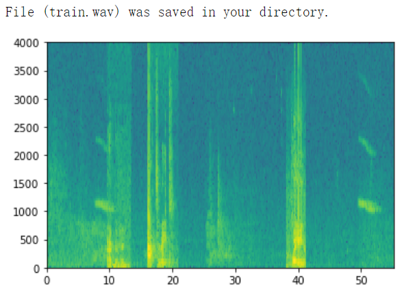
    file_handle = background.export("train" + ".wav", format="wav")
    print("File (train.wav) was saved in your directory.")
    
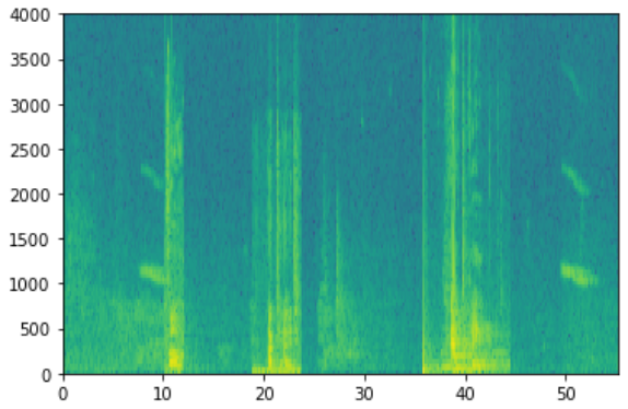
    # Get and plot spectrogram of the new recording (background with superposition of positive and negatives)
    x = graph_spectrogram("train.wav")
    
    return x, y

x, y = create_training_example(backgrounds[0], activates, negatives)

【result】

【Expected Output】

Now you can listen to the training example you created and compare it to the spectrogram generated above.

【code】

IPython.display.Audio("train.wav")

【result】

【注】原网页这背景音频里插入了两个activate,和一个非acitivate词，此处是截图。

【Expected Output】　　

　【code】

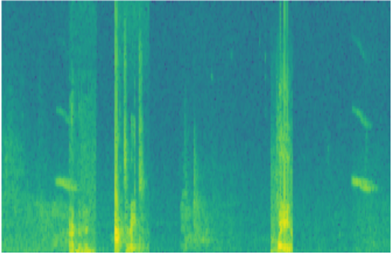
IPython.display.Audio("audio_examples/train_reference.wav")

　【注】原网页这背景音频里插入了两个activate,和一个非acitivate词，此处是截图。　

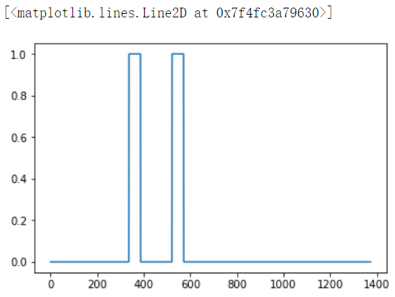
Finally, you can plot the associated labels for the generated training example.　

【code】

plt.plot(y[0])

【result】

【Expected Output】

1.4 - Full training set

You've now implemented the code needed to generate a single training example. We used this process to generate a large training set. To save time, we've already generated a set of training examples.

【code】

# Load preprocessed training examples
X = np.load("./XY_train/X.npy")
Y = np.load("./XY_train/Y.npy")

1.5 - Development set

To test our model, we recorded a development set of 25 examples. While our training data is synthesized, we want to create a development set using the same distribution as the real inputs. Thus, we recorded 25 10-second audio clips of people saying "activate" and other random words, and labeled them by hand. This follows the principle described in Course 3 that we should create the dev set to be as similar as possible to the test set distribution; that's why our dev set uses real rather than synthesized audio.

【中文翻译】　

1.5-开发集
为了测试我们的模型, 我们记录了一组25个样本的开发集。虽然我们的训练数据是合成的, 我们希望创建一个开发集，使用与实际输入相同的分布。因此, 我们记录了 25 个10 秒的音频剪辑的人说 "activate " 和其他随机词, 并手动标记他们。这遵循了课程3中描述的原则, 即我们应该创建一个与测试集分布尽可能相似的开发集;这就是为什么我们的开发集使用真正的而不是合成的音频。

【code】

# Load preprocessed dev set examples
X_dev = np.load("./XY_dev/X_dev.npy")
Y_dev = np.load("./XY_dev/Y_dev.npy")

2 - Model

Now that you've built a dataset, lets write and train a trigger word detection model!

The model will use 1-D convolutional layers, GRU layers, and dense layers. Let's load the packages that will allow you to use these layers in Keras. This might take a minute to load.

【code】

from keras.callbacks import ModelCheckpoint
from keras.models import Model, load_model, Sequential
from keras.layers import Dense, Activation, Dropout, Input, Masking, TimeDistributed, LSTM, Conv1D
from keras.layers import GRU, Bidirectional, BatchNormalization, Reshape
from keras.optimizers import Adam

2.1 - Build the model

Here is the architecture we will use. Take some time to look over the model and see if it makes sense.

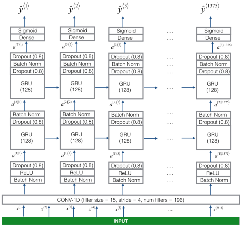
Figure 3

One key step of this model is the 1D convolutional step (near the bottom of Figure 3). It inputs the 5511 step spectrogram, and outputs a 1375 step output, which is then further processed by multiple layers to get the final

Computationally, the 1-D conv layer also helps speed up the model because now the GRU has to process only 1375 timesteps rather than 5511 timesteps. The two GRU layers read the sequence of inputs from left to right, then ultimately uses a dense+sigmoid layer to make a prediction for

Note that we use a uni-directional RNN rather than a bi-directional RNN. This is really important for trigger word detection, since we want to be able to detect the trigger word almost immediately after it is said. If we used a bi-directional RNN, we would have to wait for the whole 10sec of audio to be recorded before we could tell if "activate" was said in the first second of the audio clip.

【中文翻译】

此模型的一个关键步骤是1D 卷积步骤 (靠近图3的底部)。它输入5511步频谱图, 输出1375步输出, 然后由多个层进一步处理以获得最终的 T^y=1375步骤输出。此层扮演一个角色, 类似于您在课程4中看到的2D convolutions, 即提取低级特征, 然后可能生成较小维度的输出。

计算上, 1-D conv 层也有助于加快模型的速度, 因为现在 GRU 只能处理 1375 timesteps 而不是 5511 timesteps。两个 GRU 层从左向右读取输入序列, 最后使用一个dense+sigmoid层对 y^⟨t⟩进行预测。由于 y 是二进制值 (0 或 1), 我们使用在最后一层的sigmoid输出来估计输出为1的几率, 对应于刚才说 "activate" 的用户。

请注意, 我们使用的是单向 RNN, 而不是双向 RNN。这对于触发词检测非常重要, 因为我们希望能够在说完后立即检测到触发器词。如果我们使用双向 RNN, 我们将不得不等待整个10sec 的音频被记录, 然后我们才可以说 "activate " 是否在第一秒的音频剪辑里有说到。

Implementing the model can be done in four steps:

Step 1: CONV layer. Use Conv1D() to implement this, with 196 filters, a filter size of 15 (kernel_size=15), and stride of 4. [See documentation.]

Step 2: First GRU layer. To generate the GRU layer, use:

X = GRU(units = 128, return_sequences = True)(X)

Setting return_sequences=True ensures that all the GRU's hidden states are fed to the next layer. Remember to follow this with Dropout and BatchNorm layers.

Step 3: Second GRU layer. This is similar to the previous GRU layer (remember to use return_sequences=True), but has an extra dropout layer.

Step 4: Create a time-distributed dense layer as follows:

X = TimeDistributed(Dense(1, activation = "sigmoid"))(X)

This creates a dense layer followed by a sigmoid, so that the parameters used for the dense layer are the same for every time step. [See documentation.]

Exercise: Implement model(), the architecture is presented in Figure 3.

【中文翻译】

实现模型可以在四步骤中完成:

步骤 1: CONV 层。使用 Conv1D () 实现此目的, 使用196个过滤器, 过滤器大小为 15 (kernel_size=15), 步长为4。[请参阅文档]。

步骤 2: 第一个 GRU 层。要生成 GRU 层, 请使用:

X = GRU(units = 128, return_sequences = True)(X)

设置 return_sequences = True 可确保所有 GRU 的隐藏状态都被送入下一层。记住在这个层之后接着加Dropout和 BatchNorm 层。

步骤 3: 第二个 GRU 层。这类似于上一个 GRU 层 (记住使用 return_sequences = True), 但有一个额外的dropout层。

步骤 4: 创建一个时间分布dense层, 如下所示:

X = TimeDistributed(Dense(1, activation = "sigmoid"))(X)

这将创建一个dense层, 后跟一个 sigmoid, 因此用于dense层的参数在每一时间步中都是相同的。[请参阅文档]。

练习: 实现模型 (), 架构如图3所示。

【code】

# GRADED FUNCTION: model

def model(input_shape):
    """
    Function creating the model's graph in Keras.
    
    Argument:
    input_shape -- shape of the model's input data (using Keras conventions)

    Returns:
    model -- Keras model instance
    """
    
    X_input = Input(shape = input_shape)
    
    ### START CODE HERE ###
    
    # Step 1: CONV layer (≈4 lines)
    X = Conv1D(196, 15, strides=4)(X_input)             # CONV1D
    X = BatchNormalization()(X)                         # Batch normalization
    X = Activation('relu')(X)                           # ReLu activation
    X = Dropout(0.8)(X)                                 # dropout (use 0.8)

    # Step 2: First GRU Layer (≈4 lines)
    X = GRU(units = 128, return_sequences=True)(X)      # GRU (use 128 units and return the sequences)
    X = Dropout(0.8)(X)                                 # dropout (use 0.8)
    X = BatchNormalization()(X)                         # Batch normalization
    
    # Step 3: Second GRU Layer (≈4 lines)
    X = GRU(units = 128, return_sequences=True)(X)      # GRU (use 128 units and return the sequences)
    X = Dropout(0.8)(X)                                 # dropout (use 0.8)
    X = BatchNormalization()(X)                         # Batch normalization
    X = Dropout(0.8)(X)                                 # dropout (use 0.8)
    
    # Step 4: Time-distributed dense layer (≈1 line)
    X = TimeDistributed(Dense(1, activation = "sigmoid"))(X) # time distributed  (sigmoid)

    ### END CODE HERE ###

    model = Model(inputs = X_input, outputs = X)
    
    return model

model = model(input_shape = (Tx, n_freq))

Let's print the model summary to keep track of the shapes.

【code】

model.summary()

【result】

_________________________________________________________________
Layer (type)                 Output Shape              Param #   
=================================================================
input_1 (InputLayer)         (None, 5511, 101)         0         
_________________________________________________________________
conv1d_1 (Conv1D)            (None, 1375, 196)         297136    
_________________________________________________________________
batch_normalization_1 (Batch (None, 1375, 196)         784       
_________________________________________________________________
activation_1 (Activation)    (None, 1375, 196)         0         
_________________________________________________________________
dropout_1 (Dropout)          (None, 1375, 196)         0         
_________________________________________________________________
gru_1 (GRU)                  (None, 1375, 128)         124800    
_________________________________________________________________
dropout_2 (Dropout)          (None, 1375, 128)         0         
_________________________________________________________________
batch_normalization_2 (Batch (None, 1375, 128)         512       
_________________________________________________________________
gru_2 (GRU)                  (None, 1375, 128)         98688     
_________________________________________________________________
dropout_3 (Dropout)          (None, 1375, 128)         0         
_________________________________________________________________
batch_normalization_3 (Batch (None, 1375, 128)         512       
_________________________________________________________________
dropout_4 (Dropout)          (None, 1375, 128)         0         
_________________________________________________________________
time_distributed_1 (TimeDist (None, 1375, 1)           129       
=================================================================
Total params: 522,561
Trainable params: 521,657
Non-trainable params: 904

【Expected Output】

Total params	522,561
Trainable params	521,657
Non-trainable params	904

The output of the network is of shape (None, 1375, 1) while the input is (None, 5511, 101). The Conv1D has reduced the number of steps from 5511 at spectrogram to 1375.　　

2.2 - Fit the model

Trigger word detection takes a long time to train. To save time, we've already trained a model for about 3 hours on a GPU using the architecture you built above, and a large training set of about 4000 examples. Let's load the model.

【code】

model = load_model('./models/tr_model.h5')

You can train the model further, using the Adam optimizer and binary cross entropy loss, as follows. This will run quickly because we are training just for one epoch and with a small training set of 26 examples.　　

【code】

opt = Adam(lr=0.0001, beta_1=0.9, beta_2=0.999, decay=0.01)
model.compile(loss='binary_crossentropy', optimizer=opt, metrics=["accuracy"])

model.fit(X, Y, batch_size = 5, epochs=1)

【result】

Epoch 1/1
26/26 [==============================] - 27s - loss: 0.0726 - acc: 0.9806    
<keras.callbacks.History at 0x7f82f4fa5a58>

2.3 - Test the model

Finally, let's see how your model performs on the dev set.

【code】

loss, acc = model.evaluate(X_dev, Y_dev)
print("Dev set accuracy = ", acc)

【result】

25/25 [==============================] - 4s
Dev set accuracy =  0.945978164673

This looks pretty good! However, accuracy isn't a great metric for this task, since the labels are heavily skewed to 0's, so a neural network that just outputs 0's would get slightly over 90% accuracy. We could define more useful metrics such as F1 score or Precision/Recall. But let's not bother with that here, and instead just empirically see how the model does.　

【中文翻译】　　

这看起来不错!然而,, 对这项任务，准确性不是一个很棒的指标, 因为标签是严重扭曲到 0,。所以一个神经网络, 只是输出0的将得到略高于90% 的准确性。我们可以定义更有用的指标, 如 F1 评分或 Precision/Recall。但是, 让我们不要费心在这里, 而只是经验主义地看看模型是如何做的。　　

3 - Making Predictions

Now that you have built a working model for trigger word detection, let's use it to make predictions. This code snippet runs audio (saved in a wav file) through the network.

【中文翻译】

现在, 您已经建立了一个触发词检测的工作模型, 让我们使用它来进行预测。此代码段通过网络运行音频 (保存在 wav 文件中)。　　

【code】

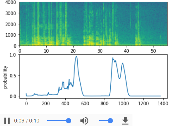
def detect_triggerword(filename):
    plt.subplot(2, 1, 1)

    x = graph_spectrogram(filename)
    # the spectogram outputs (freqs, Tx) and we want (Tx, freqs) to input into the model
    x  = x.swapaxes(0,1)
    x = np.expand_dims(x, axis=0)
    predictions = model.predict(x)
    
    plt.subplot(2, 1, 2)
    plt.plot(predictions[0,:,0])
    plt.ylabel('probability')
    plt.show()
    return predictions

Once you've estimated the probability of having detected the word "activate" at each output step, you can trigger a "chiming" sound to play when the probability is above a certain threshold. Further, 　　

【中文翻译】　　

当您估计在每个输出步骤中检测到 "activate " 这个词的概率时, 当概率高于某一阈值时, 可以触发 "chiming " 声音。此外, 在 "activate " 之后, y^⟨t⟩在一行中的许多值可能接近 1, 但我们只需要一次。因此, 我们将在每75个输出步骤中最多插入一个chiming声音。这将有助于防止我们为单一的 "activate " 实例插入两个chiming。(这与计算机视觉中的non-max suppression类似）。

【code】

chime_file = "audio_examples/chime.wav"
def chime_on_activate(filename, predictions, threshold):
    audio_clip = AudioSegment.from_wav(filename)
    chime = AudioSegment.from_wav(chime_file)
    Ty = predictions.shape[1]
    # Step 1: Initialize the number of consecutive output steps to 0 将连续输出步骤的数量初始化为0
    consecutive_timesteps = 0
    # Step 2: Loop over the output steps in the y 
    for i in range(Ty):
        # Step 3: Increment consecutive output steps 递增连续输出步骤
        consecutive_timesteps += 1
        # Step 4: If prediction is higher than the threshold and more than 75 consecutive output steps have passed 如果预测高于阈值, 超过75个连续的输出步骤已通过
        if predictions[0,i,0] > threshold and consecutive_timesteps > 75:
            # Step 5: Superpose audio and background using pydub  使用 pydub叠加音频和背景
            audio_clip = audio_clip.overlay(chime, position = ((i / Ty) * audio_clip.duration_seconds)*1000)
            # Step 6: Reset consecutive output steps to 0   将连续的输出步骤重置为0
            consecutive_timesteps = 0
        
    audio_clip.export("chime_output.wav", format='wav')

3.3 - Test on dev examples]

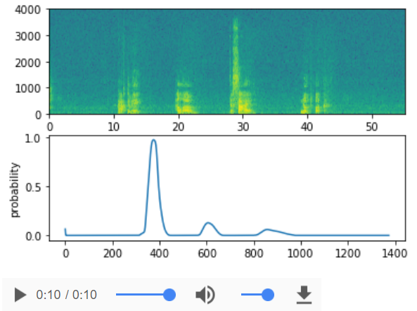
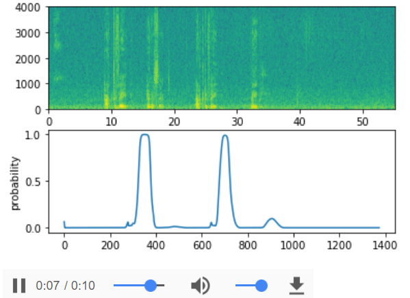
Let's explore how our model performs on two unseen audio clips from the development set. Lets first listen to the two dev set clips.

【code】

IPython.display.Audio("./raw_data/dev/1.wav")

【result】

【注】原文是音频，这里第截图

【code】

IPython.display.Audio("./raw_data/dev/2.wav")

【result】　　

【注】原文是音频，这里第截图

Now lets run the model on these audio clips and see if it adds a chime after "activate"!

【code】

filename = "./raw_data/dev/1.wav"
prediction = detect_triggerword(filename)
chime_on_activate(filename, prediction, 0.5)
IPython.display.Audio("./chime_output.wav")

【result】

【code】

filename  = "./raw_data/dev/2.wav"
prediction = detect_triggerword(filename)
chime_on_activate(filename, prediction, 0.5)
IPython.display.Audio("./chime_output.wav")

【result】　　

Congratulations

You've come to the end of this assignment!

Here's what you should remember:

Data synthesis is an effective way to create a large training set for speech problems, specifically trigger word detection.
Using a spectrogram and optionally a 1D conv layer is a common pre-processing step prior to passing audio data to an RNN, GRU or LSTM.
An end-to-end deep learning approach can be used to built a very effective trigger word detection system.

Congratulations on finishing the fimal assignment!

Thank you for sticking with us through the end and for all the hard work you've put into learning deep learning. We hope you have enjoyed the course!

【中文翻译】

祝贺
你已经完成任务了!

以下是你应该记住的:

数据合成是创建一个用于语音问题的大型训练集的有效方法, 特别是触发词检测。
在将音频数据传递给 RNN、GRU 或 LSTM 之前, 使用频谱图和可选的 1D conv 层是一个常见的预处理步骤。
端到端的深层学习方法可以用来构建一个非常有效的触发词检测系统。

恭喜你完成了 fimal 任务!

谢谢你跟着我们坚持到最后以及你所有的辛勤工作, 你已经投入到学习深入学习。我们希望你喜欢这门课!

4 - Try your own example! (OPTIONAL/UNGRADED)

In this optional and ungraded portion of this notebook, you can try your model on your own audio clips!

Record a 10 second audio clip of you saying the word "activate" and other random words, and upload it to the Coursera hub as myaudio.wav. Be sure to upload the audio as a wav file. If your audio is recorded in a different format (such as mp3) there is free software that you can find online for converting it to wav. If your audio recording is not 10 seconds, the code below will either trim or pad it as needed to make it 10 seconds.

【中文翻译】

4-尝试你自己的例子!(可选/不评分)
在本笔记本的这个可选和不评分的部分中, 您可以在自己的音频剪辑上试用您的模型!

记录一个10秒的音频剪辑, 你说的字 "activate " 和其他随机词, 并上传到 Coursera hub作为 myaudio. wav。请务必将音频上载为 wav 文件。如果您的音频以不同的格式 (如 mp3) 录制, 则可以在联网状态下找到用于将其转换为 wav 的免费软件。如果您的录音不是10秒, 下面的代码将根据需要修剪或填充它, 使其10秒。

【code】

# Preprocess the audio to the correct format
def preprocess_audio(filename):
    # Trim or pad audio segment to 10000ms
    padding = AudioSegment.silent(duration=10000)
    segment = AudioSegment.from_wav(filename)[:10000]
    segment = padding.overlay(segment)
    # Set frame rate to 44100
    segment = segment.set_frame_rate(44100)
    # Export as wav
    segment.export(filename, format='wav')

Once you've uploaded your audio file to Coursera, put the path to your file in the variable below.

【code】

your_filename = "audio_examples/my_audio.wav"

preprocess_audio(your_filename)
IPython.display.Audio(your_filename) # listen to the audio you uploaded

【result】

【注】原文是音频，这里第截图

Finally, use the model to predict when you say activate in the 10 second audio clip, and trigger a chime. If beeps are not being added appropriately, try to adjust the chime_threshold.　　

【中文翻译】

最后, 使用模型预测当您在第二个10s音频剪辑中说activate, 并触发一个chime。如果未正确添加chime, 请尝试调整 chime_threshold。

【code】

chime_threshold = 0.5
prediction = detect_triggerword(your_filename)
chime_on_activate(your_filename, prediction, chime_threshold)
IPython.display.Audio("./chime_output.wav")

【result】