课程四(Convolutional Neural Networks)，第四周（Special applications: Face recognition & Neural style transfer） —— 2.Programming assignments：Art generation with Neural Style Transfer

Deep Learning & Art: Neural Style Transfer

Welcome to the second assignment of this week. In this assignment, you will learn about Neural Style Transfer. This algorithm was created by Gatys et al. (2015) (https://arxiv.org/abs/1508.06576).

In this assignment, you will:

Implement the neural style transfer algorithm
Generate novel artistic images using your algorithm

Most of the algorithms you've studied optimize a cost function to get a set of parameter values. In Neural Style Transfer, you'll optimize a cost function to get pixel values!

【中文翻译】

深度学习与艺术: 神经风格转换

欢迎来到这周的第二次任务。在这个作业中, 您将了解到神经风格的转换。该算法 (https://arxiv.org/abs/1508.06576)是由 Gatys 等 (2015) 创建的。

在该任务中, 您将:

实现神经风格转换算法
使用您的算法生成新的艺术图像

您研究的大多数算法都优化了成本函数以获得一组参数值。在神经风格传输中, 您将优化成本函数以获得像素值!

【code】

import os
import sys
import scipy.io
import scipy.misc
import matplotlib.pyplot as plt
from matplotlib.pyplot import imshow
from PIL import Image
from nst_utils import *
import numpy as np
import tensorflow as tf

%matplotlib inline

1 - Problem Statement

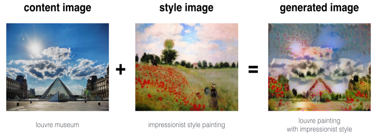
Neural Style Transfer (NST) is one of the most fun techniques in deep learning. As seen below, it merges two images, namely, a "content" image (C) and a "style" image (S), to create a "generated" image (G). The generated image G combines the "content" of the image C with the "style" of image S.

In this example, you are going to generate an image of the Louvre museum in Paris (content image C), mixed with a painting by Claude Monet, a leader of the impressionist movement (style image S).

Let's see how you can do this.

【中文翻译】　

1-问题声明

神经风格转换 (NST) 是深部学习中最有趣的技术之一。如下所示, 它合并两个图像, 即 "内容" 图像 C 和 "样式" 图像S, 以创建 "生成的" 图像 G。生成的图像 G 将图像 C 的 "内容" 与图像S的 "样式" 组合在一起。

在这个例子中, 你将产生一个图片, 由巴黎卢浮宫博物馆 (内容图像 C)混合一幅由一个的印象派运动的领导者Claude Monet的画(风格形象 S)而成。

图片见英文部分

让我们看看你怎么能做到这一点。

2 - Transfer Learning

Neural Style Transfer (NST) uses a previously trained convolutional network, and builds on top of that. The idea of using a network trained on a different task and applying it to a new task is called transfer learning.

Following the original NST paper (https://arxiv.org/abs/1508.06576), we will use the VGG network. Specifically, we'll use VGG-19, a 19-layer version of the VGG network. This model has already been trained on the very large ImageNet database, and thus has learned to recognize a variety of low level features (at the earlier layers) and high level features (at the deeper layers).

Run the following code to load parameters from the VGG model. This may take a few seconds.

【code】

model = load_vgg_model("pretrained-model/imagenet-vgg-verydeep-19.mat")
print(model)

【result】

{'input': <tf.Variable 'Variable:0' shape=(1, 300, 400, 3) dtype=float32_ref>,
 'conv1_1': <tf.Tensor 'Relu:0' shape=(1, 300, 400, 64) dtype=float32>, 
 'conv1_2': <tf.Tensor 'Relu_1:0' shape=(1, 300, 400, 64) dtype=float32>,
 'avgpool1': <tf.Tensor 'AvgPool:0' shape=(1, 150, 200, 64) dtype=float32>,
 'conv2_1': <tf.Tensor 'Relu_2:0' shape=(1, 150, 200, 128) dtype=float32>, 
 'conv2_2': <tf.Tensor 'Relu_3:0' shape=(1, 150, 200, 128) dtype=float32>, 
 'avgpool2': <tf.Tensor 'AvgPool_1:0' shape=(1, 75, 100, 128) dtype=float32>, 
 'conv3_1': <tf.Tensor 'Relu_4:0' shape=(1, 75, 100, 256) dtype=float32>, 
 'conv3_2': <tf.Tensor 'Relu_5:0' shape=(1, 75, 100, 256) dtype=float32>, 
 'conv3_3': <tf.Tensor 'Relu_6:0' shape=(1, 75, 100, 256) dtype=float32>, 
 'conv3_4': <tf.Tensor 'Relu_7:0' shape=(1, 75, 100, 256) dtype=float32>,
 'avgpool3': <tf.Tensor 'AvgPool_2:0' shape=(1, 38, 50, 256) dtype=float32>,
 'conv4_1': <tf.Tensor 'Relu_8:0' shape=(1, 38, 50, 512) dtype=float32>, 
 'conv4_2': <tf.Tensor 'Relu_9:0' shape=(1, 38, 50, 512) dtype=float32>, 
 'conv4_3': <tf.Tensor 'Relu_10:0' shape=(1, 38, 50, 512) dtype=float32>, 
 'conv4_4': <tf.Tensor 'Relu_11:0' shape=(1, 38, 50, 512) dtype=float32>, 
 'avgpool4': <tf.Tensor 'AvgPool_3:0' shape=(1, 19, 25, 512) dtype=float32>, 
 'conv5_1': <tf.Tensor 'Relu_12:0' shape=(1, 19, 25, 512) dtype=float32>, 
 'conv5_2': <tf.Tensor 'Relu_13:0' shape=(1, 19, 25, 512) dtype=float32>,
 'conv5_3': <tf.Tensor 'Relu_14:0' shape=(1, 19, 25, 512) dtype=float32>,
 'conv5_4': <tf.Tensor 'Relu_15:0' shape=(1, 19, 25, 512) dtype=float32>,
 'avgpool5': <tf.Tensor 'AvgPool_4:0' shape=(1, 10, 13, 512) dtype=float32>}

The model is stored in a python dictionary where each variable name is the key and the corresponding value is a tensor containing that variable's value. To run an image through this network, you just have to feed the image to the model. In TensorFlow, you can do so using the tf.assign function. In particular, you will use the assign function like this:　　

【code】

model["input"].assign(image)

This assigns the image as an input to the model. After this, if you want to access the activations of a particular layer, say layer 4_2 when the network is run on this image, you would run a TensorFlow session on the correct tensor conv4_2, as follows:

【code】　　

sess.run(model["conv4_2"])

【中文翻译】

2-迁移学习

神经风格转换 (NST) 使用以前经过训练的卷积网络, 并建立在上面。使用对不同任务进行培训的网络并将其应用于新任务的想法称为迁移学习。

继原 NST 论文 (https://arxiv.org/abs/1508.06576) 后, 我们将使用 VGG 网络。具体地说, 我们将使用 VGG-19, 一个19层版本的 VGG 网络。此模型已经在非常大的 ImageNet 数据库上进行了训练, 因此学会了识别各种低级特征 (在较早的层) 和高级特征 (在更深层)。

运行以下代码从 VGG 模型加载参数。这可能需要几秒钟。

【code】

model = load_vgg_model("pretrained-model/imagenet-vgg-verydeep-19.mat")
print(model)

【result】　　

{'input': <tf.Variable 'Variable:0' shape=(1, 300, 400, 3) dtype=float32_ref>,
 'conv1_1': <tf.Tensor 'Relu:0' shape=(1, 300, 400, 64) dtype=float32>, 
 'conv1_2': <tf.Tensor 'Relu_1:0' shape=(1, 300, 400, 64) dtype=float32>,
 'avgpool1': <tf.Tensor 'AvgPool:0' shape=(1, 150, 200, 64) dtype=float32>,
 'conv2_1': <tf.Tensor 'Relu_2:0' shape=(1, 150, 200, 128) dtype=float32>, 
 'conv2_2': <tf.Tensor 'Relu_3:0' shape=(1, 150, 200, 128) dtype=float32>, 
 'avgpool2': <tf.Tensor 'AvgPool_1:0' shape=(1, 75, 100, 128) dtype=float32>, 
 'conv3_1': <tf.Tensor 'Relu_4:0' shape=(1, 75, 100, 256) dtype=float32>, 
 'conv3_2': <tf.Tensor 'Relu_5:0' shape=(1, 75, 100, 256) dtype=float32>, 
 'conv3_3': <tf.Tensor 'Relu_6:0' shape=(1, 75, 100, 256) dtype=float32>, 
 'conv3_4': <tf.Tensor 'Relu_7:0' shape=(1, 75, 100, 256) dtype=float32>,
 'avgpool3': <tf.Tensor 'AvgPool_2:0' shape=(1, 38, 50, 256) dtype=float32>,
 'conv4_1': <tf.Tensor 'Relu_8:0' shape=(1, 38, 50, 512) dtype=float32>, 
 'conv4_2': <tf.Tensor 'Relu_9:0' shape=(1, 38, 50, 512) dtype=float32>, 
 'conv4_3': <tf.Tensor 'Relu_10:0' shape=(1, 38, 50, 512) dtype=float32>, 
 'conv4_4': <tf.Tensor 'Relu_11:0' shape=(1, 38, 50, 512) dtype=float32>, 
 'avgpool4': <tf.Tensor 'AvgPool_3:0' shape=(1, 19, 25, 512) dtype=float32>, 
 'conv5_1': <tf.Tensor 'Relu_12:0' shape=(1, 19, 25, 512) dtype=float32>, 
 'conv5_2': <tf.Tensor 'Relu_13:0' shape=(1, 19, 25, 512) dtype=float32>,
 'conv5_3': <tf.Tensor 'Relu_14:0' shape=(1, 19, 25, 512) dtype=float32>,
 'conv5_4': <tf.Tensor 'Relu_15:0' shape=(1, 19, 25, 512) dtype=float32>,
 'avgpool5': <tf.Tensor 'AvgPool_4:0' shape=(1, 10, 13, 512) dtype=float32>}

模型存储在 python 字典中, 其中每个变量名都是key, 对应的值是包含该变量值的tensor。若要通过此网络运行图像, 只需将图像提供给模型。在 TensorFlow 中, 您可以使用 tf.assign函数。特别地, 您将使用如下所指的赋值函数:　

【code】

model["input"].assign(image)

这会将图像分配给模型的输入。在此之后, 如果要访问特定层的激活值, 请在该图像上运行网络时说 "layer 4_2", 则在正确的tensor conv4_2 上运行 TensorFlow session, 如下所示:　　

【code】　

sess.run(model["conv4_2"])

3 - Neural Style Transfer

We will build the NST algorithm in three steps:

Build the content cost function
Build the style cost function
Put it together to get

3.1 - Computing the content cost

In our running example, the content image C will be the picture of the Louvre Museum in Paris. Run the code below to see a picture of the Louvre.

【code】

content_image = scipy.misc.imread("images/louvre.jpg")
imshow(content_image)

【result】

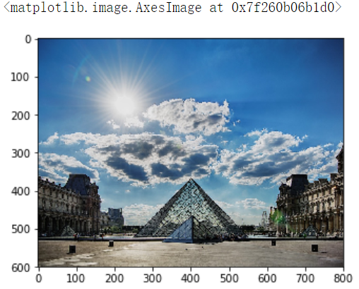
The content image (C) shows the Louvre museum's pyramid surrounded by old Paris buildings, against a sunny sky with a few clouds.

3.1.1 - How do you ensure the generated image G matches the content of the image C?

As we saw in lecture, the earlier (shallower) layers of a ConvNet tend to detect lower-level features such as edges and simple textures, and the later (deeper) layers tend to detect higher-level features such as more complex textures as well as object classes.

We would like the "generated" image G to have similar content as the input image C. Suppose you have chosen some layer's activations to represent the content of an image. In practice, you'll get the most visually pleasing results if you choose a layer in the middle of the network--neither too shallow nor too deep. (After you have finished this exercise, feel free to come back and experiment with using different layers, to see how the results vary.)

So, suppose you have picked one particular hidden layer to use. Now, set the image C as the input to the pretrained VGG network, and run forward propagation. Let $a^{(G)}$ be the corresponding hidden layer activation. We will define as the content cost function as:

Here,

【中文翻译】

3.1.1-如何确保生成的图像 G 与图像 C 的内容匹配

正如我们在讲座中看到的, 早期 (较浅) 的 ConvNet 层倾向于检测较低级别的特征, 如边缘和简单纹理, 而以后 (更深的) 图层则倾向于检测更高级的特征, 如更复杂的纹理以及对象的类别。

我们希望 "生成的" 图像 G与输入图像C 具有类似的内容。 假设您选择了某层的激活值来表示图像的内容。在实践中, 如果你选择网络中间的一层, 你会得到最直观的结果--既不太浅也不太深。(完成此练习后, 请随时返回并尝试使用不同的图层, 查看结果的变化情况。）

因此, 假设您选择了一个特定的隐藏层来使用。现在, 将图像 C 设置为预先训练好的VGG 网络的输入, 并运行向前传播。让 a ^(C) 成为您选择的隐藏层的激活值。(在视频中, 我们写成 a^[l](C), 但在这里我们将删除上标 [l] 以简化表示法。这将是一个n_H×n_W×n_C 张量。重复此过程与图像 G: 设置 G 为输入, 并运行前向传播。让 a^(G)成为相应的隐藏层激活值。我们将定义为内容成本函数为:

这里, n_H、n_W 和 n_C 是您选择的隐藏层的高度、宽度和通道数, 并在成本中显示为标准化的值。为清楚起见, 请注意, a^(C) 和 a^(G) 是与隐藏层的激活值相对应的volume。为了计算成本 J_content (C, G), 也可以方便地将这些3D volume展开为2D matrix, 如下所示。(技术上这展开步骤不需要计算 Jcontent, 但在以后需要执行类似的操作以计算样式常量 Jstyle 时, 这将是一个很好的实践。）

Exercise: Compute the "content cost" using TensorFlow.

Instructions: The 3 steps to implement this function are:

Retrieve dimensions from a_G:
- To retrieve dimensions from a tensor X, use: X.get_shape().as_list()
Unroll a_C and a_G as explained in the picture above
- If you are stuck, take a look at Hint1 and Hint2.
Compute the content cost:
- If you are stuck, take a look at Hint3, Hint4 and Hint5.

【code】

# GRADED FUNCTION: compute_content_cost

def compute_content_cost(a_C, a_G):
    """
    Computes the content cost
    
    Arguments:
    a_C -- tensor of dimension (1, n_H, n_W, n_C), hidden layer activations representing content of the image C 
    a_G -- tensor of dimension (1, n_H, n_W, n_C), hidden layer activations representing content of the image G
    
    Returns: 
    J_content -- scalar that you compute using equation 1 above.
    """
    
    ### START CODE HERE ###
    # Retrieve dimensions from a_G (≈1 line)
    m, n_H, n_W, n_C =  a_G.get_shape().as_list()
    
    # Reshape a_C and a_G (≈2 lines)
    a_C_unrolled = tf.reshape(tf.transpose(a_C, perm=[3, 1, 2, 0]), [n_C, n_H*n_W, -1]) # tanspose后a_C的维度(n_C,n_H, n_W,1)
    a_G_unrolled = tf.reshape(tf.transpose(a_G, perm=[3, 1, 2, 0]), [n_C, n_H*n_W, -1]) # tanspose后a_G的维度(n_C,n_H, n_W,1)
    
    # compute the cost with tensorflow (≈1 line)
    J_content =  tf.reduce_sum(tf.square(tf.subtract(a_C_unrolled, a_G_unrolled))) / (4 * n_H * n_W * n_C)
    ### END CODE HERE ###
    
    return J_content

tf.reset_default_graph()

with tf.Session() as test:
    tf.set_random_seed(1)
    a_C = tf.random_normal([1, 4, 4, 3], mean=1, stddev=4)
    a_G = tf.random_normal([1, 4, 4, 3], mean=1, stddev=4)
    J_content = compute_content_cost(a_C, a_G)
    print("J_content = " + str(J_content.eval()))

【result】

J_content = 6.76559

Expected Output:

J_content

6.76559

What you should remember:

The content cost takes a hidden layer activation of the neural network, and measures how different
When we minimize the content cost later, this will help make sure

3.2 - Computing the style cost

For our running example, we will use the following style image:

【code】

style_image = scipy.misc.imread("images/monet_800600.jpg")
imshow(style_image)

【result】　　

This painting was painted in the style of impressionism（印象派）.

Lets see how you can now define a "style" const function

3.2.1 - Style matrix

The style matrix is also called a "Gram matrix." In linear algebra, the Gram matrix G of a set of vectors

Note that there is an unfortunate collision in the variable names used here. We are following common terminology used in the literature, but

In NST, you can compute the Style matrix by multiplying the "unrolled" filter matrix with their transpose:

The result is a matrix of dimension

One important part of the gram matrix is that the diagonal elements such as

By capturing the prevalence of different types of features (

【中文翻译】

3.2.1 风格矩阵

风格矩阵也称为 "Gram矩阵"。在线性代数中, 一组向量

的Gram矩阵 G 是点积的矩阵, 其内容是

。换言之, G_ij 比较了v_i和

的相似之处在: 如果它们高度相似, 你会期望他们有一个大点的 dot product, 因此 G_ij 是大的。

请注意, 此处使用的变量名发生了不幸的冲突。我们遵循文献中常用的术语, 但 G 用于表示样式矩阵 (或Gram矩阵) 以及表示生成的图像 G。我们将尽力确保我们所指的 G 从上下文中始终是清晰的。

在 NST 中, 可以通过将 "unrolled" filter matrix与其转置相乘来计算样式矩阵:

结果是一个维度为 (n_C,n_C)的矩阵, 其中 n_C是过滤器的数量。值 G_ij 度量过滤器i的激活值与筛选器 j 的激活值的相似程度。

Gram矩阵的一个重要部分是, 诸如 G_ii 等对角线元素也测量了过滤器的激活程度。例如, 假设过滤器 i 正在检测图像中的垂直纹理。然后,G_ii 测量了整个图像中的垂直纹理: 如果G_ii 很大, 这意味着图像有很多垂直纹理。

通过捕获不同类型的特征 (G_ii) , 以及在一起有多少不同的特征 (Gij), 样式矩阵 G 度量图像的样式。

Exercise: Using TensorFlow, implement a function that computes the Gram matrix of a matrix A. The formula is: The gram matrix of A is

【code】

# GRADED FUNCTION: gram_matrix

def gram_matrix(A):
    """
    Argument:
    A -- matrix of shape (n_C, n_H*n_W)
    
    Returns:
    GA -- Gram matrix of A, of shape (n_C, n_C)
    """
    
    ### START CODE HERE ### (≈1 line)
    GA = tf.matmul(A,tf.transpose(A))
    ### END CODE HERE ###
    
    return GA

tf.reset_default_graph()

with tf.Session() as test:
    tf.set_random_seed(1)
    A = tf.random_normal([3, 2*1], mean=1, stddev=4)
    GA = gram_matrix(A)
    
    print("GA = " + str(GA.eval()))

【result】

GA = [[  6.42230511  -4.42912197  -2.09668207]
 [ -4.42912197  19.46583748  19.56387138]
 [ -2.09668207  19.56387138  20.6864624 ]]

Expected Output:

GA	[[ 6.42230511 -4.42912197 -2.09668207] [ -4.42912197 19.46583748 19.56387138] [ -2.09668207 19.56387138 20.6864624 ]]

3.2.2 - Style cost

After generating the Style matrix (Gram matrix), your goal will be to minimize the distance between the Gram matrix of the "style" image S and that of the "generated" image G. For now, we are using only a single hidden layer

where

Exercise: Compute the style cost for a single layer.

Instructions: The 3 steps to implement this function are:

Retrieve dimensions from the hidden layer activations a_G:
- To retrieve dimensions from a tensor X, use: X.get_shape().as_list()
Unroll the hidden layer activations a_S and a_G into 2D matrices, as explained in the picture above.
- You may find Hint1 and Hint2 useful.
Compute the Style matrix of the images S and G. (Use the function you had previously written.)
Compute the Style cost:
- You may find Hint3, Hint4 and Hint5 useful.

【code】　　

# GRADED FUNCTION: compute_layer_style_cost

def compute_layer_style_cost(a_S, a_G):
    """
    Arguments:
    a_S -- tensor of dimension (1, n_H, n_W, n_C), hidden layer activations representing style of the image S 
    a_G -- tensor of dimension (1, n_H, n_W, n_C), hidden layer activations representing style of the image G
    
    Returns: 
    J_style_layer -- tensor representing a scalar value, style cost defined above by equation (2)
    """
    
    ### START CODE HERE ###
    # Retrieve dimensions from a_G (≈1 line)
    m, n_H, n_W, n_C =a_G.get_shape().as_list()
    
    # Reshape the images to have them of shape (n_C, n_H*n_W) (≈2 lines)
    a_S = tf.reshape(tf.transpose(a_S, perm=[3, 1, 2, 0]), [n_C, n_W*n_H])
    a_G = tf.reshape(tf.transpose(a_G, perm=[3, 1, 2, 0]), [n_C, n_W*n_H])

    # Computing gram_matrices for both images S and G (≈2 lines)
    GS = gram_matrix(a_S)
    GG = gram_matrix(a_G)

    # Computing the loss (≈1 line)
    J_style_layer = tf.reduce_sum(tf.square(tf.subtract(GS, GG))) / (4 * n_C**2 * (n_W * n_H)**2)
    
    ### END CODE HERE ###
    
    return J_style_layer

tf.reset_default_graph()

with tf.Session() as test:
    tf.set_random_seed(1)
    a_S = tf.random_normal([1, 4, 4, 3], mean=1, stddev=4)
    a_G = tf.random_normal([1, 4, 4, 3], mean=1, stddev=4)
    J_style_layer = compute_layer_style_cost(a_S, a_G)
    
    print("J_style_layer = " + str(J_style_layer.eval()))

【result】

J_style_layer = 9.19028

Expected Output:

J_style_layer

9.19028

3.2.3 Style Weights

So far you have captured the style from only one layer. We'll get better results if we "merge" style costs from several different layers. After completing this exercise, feel free to come back and experiment with different weights to see how it changes the generated image

【code】

STYLE_LAYERS = [
    ('conv1_1', 0.2),
    ('conv2_1', 0.2),
    ('conv3_1', 0.2),
    ('conv4_1', 0.2),
    ('conv5_1', 0.2)]

You can combine the style costs for different layers as follows:　　

where the values for

We've implemented a compute_style_cost(...) function. It simply calls your compute_layer_style_cost(...) several times, and weights their results using the values in STYLE_LAYERS. Read over it to make sure you understand what it's doing.　　

【code】

def compute_style_cost(model, STYLE_LAYERS):
    """
    Computes the overall style cost from several chosen layers
    
    Arguments:
    model -- our tensorflow model
    STYLE_LAYERS -- A python list containing:
                        - the names of the layers we would like to extract style from
                        - a coefficient for each of them
    
    Returns: 
    J_style -- tensor representing a scalar value, style cost defined above by equation (2)
    """
    
    # initialize the overall style cost
    J_style = 0

    for layer_name, coeff in STYLE_LAYERS:

        # Select the output tensor of the currently selected layer
        out = model[layer_name]

        # Set a_S to be the hidden layer activation from the layer we have selected, by running the session on out
        a_S = sess.run(out)

        # Set a_G to be the hidden layer activation from same layer. Here, a_G references model[layer_name] 
        # and isn't evaluated yet. Later in the code, we'll assign the image G as the model input, so that
        # when we run the session, this will be the activations drawn from the appropriate layer, with G as input.
        a_G = out
        
        # Compute style_cost for the current layer
        J_style_layer = compute_layer_style_cost(a_S, a_G)

        # Add coeff * J_style_layer of this layer to overall style cost
        J_style += coeff * J_style_layer

    return J_style

Note: In the inner-loop of the for-loop above, a_G is a tensor and hasn't been evaluated yet. It will be evaluated and updated at each iteration when we run the TensorFlow graph in model_nn() below.

What you should remember:

The style of an image can be represented using the Gram matrix of a hidden layer's activations. However, we get even better results combining this representation from multiple different layers. This is in contrast to the content representation, where usually using just a single hidden layer is sufficient.
Minimizing the style cost will cause the image

3.3 - Defining the total cost to optimize

Finally, let's create a cost function that minimizes both the style and the content cost. The formula is:　　

Exercise: Implement the total cost function which includes both the content cost and the style cost.

【code】

# GRADED FUNCTION: total_cost

def total_cost(J_content, J_style, alpha = 10, beta = 40):
    """
    Computes the total cost function
    
    Arguments:
    J_content -- content cost coded above
    J_style -- style cost coded above
    alpha -- hyperparameter weighting the importance of the content cost
    beta -- hyperparameter weighting the importance of the style cost
    
    Returns:
    J -- total cost as defined by the formula above.
    """
    
    ### START CODE HERE ### (≈1 line)
    J =  alpha*J_content + beta*J_style
    ### END CODE HERE ###
    
    return J

tf.reset_default_graph()

with tf.Session() as test:
    np.random.seed(3)
    J_content = np.random.randn()    
    J_style = np.random.randn()
    J = total_cost(J_content, J_style)
    print("J = " + str(J))

【result】

J = 35.34667875478276

Expected Output:

J	35.34667875478276

What you should remember:

The total cost is a linear combination of the content cost

4 - Solving the optimization problem

Finally, let's put everything together to implement Neural Style Transfer!

Here's what the program will have to do:

Create an Interactive Session
Load the content image
Load the style image
Randomly initialize the image to be generated
Load the VGG19 model
Build the TensorFlow graph:
- Run the content image through the VGG19 model and compute the content cost
- Run the style image through the VGG19 model and compute the style cost
- Compute the total cost
- Define the optimizer and the learning rate
Initialize the TensorFlow graph and run it for a large number of iterations, updating the generated image at every step.

Lets go through the individual steps in detail.

You've previously implemented the overall cost 　　

【中文翻译】　　

最后, 让我们把一切都放在一起来实现神经风格的传递!

以下是该程序将必须执行的操作:

创建交互式会话
加载内容图像
加载样式图像
随机初始化要生成的图像
加载 VGG19 模型
生成 TensorFlow 图:
- 　　通过 VGG19 模型运行内容映像并计算内容成本
- 　　通过 VGG19 模型运行样式图像并计算样式成本
- 　　计算总成本
- 　　定义优化器和学习率
初始化 TensorFlow 图并为大量的迭代运行它, 并在每个步骤中更新生成的图像。

让我们详细地浏览各个步骤。

您以前实现了总成本 j (G) 。现在, 我们将建立 TensorFlow, 以优化该成本函数。为此, 您的程序必须重置图并使用 "交互式会话"。与常规会话不同, "交互式会话" 将自身安装为用于生成图的默认会话。这允许在不必经常需要引用会话对象的情况下，运行变量, 从而简化了代码。　　

Lets start the interactive session.

【code】

# Reset the graph
tf.reset_default_graph()

# Start interactive session
sess = tf.InteractiveSession()

Let's load, reshape, and normalize our "content" image (the Louvre museum picture):　　

【code】

content_image = scipy.misc.imread("images/louvre_small.jpg")
content_image = reshape_and_normalize_image(content_image)

Let's load, reshape and normalize our "style" image (Claude Monet's painting):

【code】

style_image = scipy.misc.imread("images/monet.jpg")
style_image = reshape_and_normalize_image(style_image)

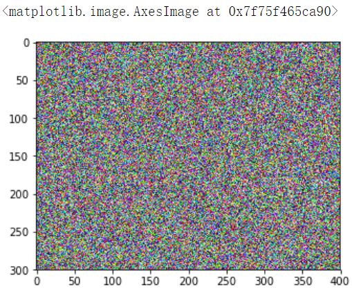
Now, we initialize the "generated" image as a noisy image created from the content_image. By initializing the pixels of the generated image to be mostly noise but still slightly correlated with the content image, this will help the content of the "generated" image more rapidly match the content of the "content" image. (Feel free to look in nst_utils.py to see the details of generate_noise_image(...); to do so, click "File-->Open..." at the upper-left corner of this Jupyter notebook.)　　

【code】

generated_image = generate_noise_image(content_image)
imshow(generated_image[0])

【result】

Next, as explained in part (2), let's load the VGG16 model.

【code】

model = load_vgg_model("pretrained-model/imagenet-vgg-verydeep-19.mat")

To get the program to compute the content cost, we will now assign a_C and a_G to be the appropriate hidden layer activations. We will use layer conv4_2 to compute the content cost. The code below does the following:

Assign the content image to be the input to the VGG model.
Set a_C to be the tensor giving the hidden layer activation for layer "conv4_2".
Set a_G to be the tensor giving the hidden layer activation for the same layer.
Compute the content cost using a_C and a_G.

【code】

# Assign the content image to be the input of the VGG model.  
sess.run(model['input'].assign(content_image))

# Select the output tensor of layer conv4_2
out = model['conv4_2']

# Set a_C to be the hidden layer activation from the layer we have selected
a_C = sess.run(out)

# Set a_G to be the hidden layer activation from same layer. Here, a_G references model['conv4_2'] 
# and isn't evaluated yet. Later in the code, we'll assign the image G as the model input, so that
# when we run the session, this will be the activations drawn from the appropriate layer, with G as input.
a_G = out

# Compute the content cost
J_content = compute_content_cost(a_C, a_G)

Note: At this point, a_G is a tensor and hasn't been evaluated. It will be evaluated and updated at each iteration when we run the Tensorflow graph in model_nn() below.　　

【code】

# Assign the input of the model to be the "style" image 
sess.run(model['input'].assign(style_image))

# Compute the style cost
J_style = compute_style_cost(model, STYLE_LAYERS)

Exercise: Now that you have J_content and J_style, compute the total cost J by calling total_cost(). Use alpha = 10 and beta = 40.　　

【code】

### START CODE HERE ### (1 line)
J =total_cost(J_content, J_style, alpha = 10, beta = 40)
### END CODE HERE ###

You'd previously learned how to set up the Adam optimizer in TensorFlow. Lets do that here, using a learning rate of 2.0. See reference　　

【code】

# define optimizer (1 line)
optimizer = tf.train.AdamOptimizer(2.0)

# define train_step (1 line)
train_step = optimizer.minimize(J)

Exercise: Implement the model_nn() function which initializes the variables of the tensorflow graph, assigns the input image (initial generated image) as the input of the VGG19 model and runs the train_step for a large number of steps.　

ef model_nn(sess, input_image, num_iterations = 200):
    
    # Initialize global variables (you need to run the session on the initializer)
    ### START CODE HERE ### (1 line)
    sess.run(tf.global_variables_initializer())
    ### END CODE HERE ###
    
    # Run the noisy input image (initial generated image) through the model. Use assign().
    ### START CODE HERE ### (1 line)
    sess.run(model['input'].assign(input_image))
    ### END CODE HERE ###
    
    for i in range(num_iterations):
    
        # Run the session on the train_step to minimize the total cost
        ### START CODE HERE ### (1 line)
        sess.run(train_step)
        ### END CODE HERE ###
        
        # Compute the generated image by running the session on the current model['input']
        ### START CODE HERE ### (1 line)
        generated_image = sess.run(model['input'])
        ### END CODE HERE ###

        # Print every 20 iteration.
        if i%20 == 0:
            Jt, Jc, Js = sess.run([J, J_content, J_style])
            print("Iteration " + str(i) + " :")
            print("total cost = " + str(Jt))
            print("content cost = " + str(Jc))
            print("style cost = " + str(Js))
            
            # save current generated image in the "/output" directory
            save_image("output/" + str(i) + ".png", generated_image)
    
    # save last generated image
    save_image('output/generated_image.jpg', generated_image)
    
    return generated_image

Run the following cell to generate an artistic image. It should take about 3min on CPU for every 20 iterations but you start observing attractive results after ≈140 iterations. Neural Style Transfer is generally trained using GPUs.　　

【co'de】

model_nn(sess, generated_image)

【result】

Iteration 0 :
total cost = 5.05035e+09
content cost = 7877.67
style cost = 1.26257e+08

Expected Output:

Iteration 0 :

total cost = 5.05035e+09
content cost = 7877.67
style cost = 1.26257e+08

You're done! After running this, in the upper bar of the notebook click on "File" and then "Open". Go to the "/output" directory to see all the saved images. Open "generated_image" to see the generated image! :)

You should see something the image presented below on the right:

We didn't want you to wait too long to see an initial result, and so had set the hyperparameters accordingly. To get the best looking results, running the optimization algorithm longer (and perhaps with a smaller learning rate) might work better. After completing and submitting this assignment, we encourage you to come back and play more with this notebook, and see if you can generate even better looking images.

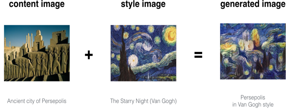
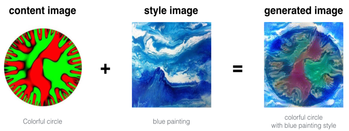
Here are few other examples:

The beautiful ruins of the ancient city of Persepolis (Iran) with the style of Van Gogh (The Starry Night)

The tomb of Cyrus the great in Pasargadae with the style of a Ceramic Kashi from Ispahan.

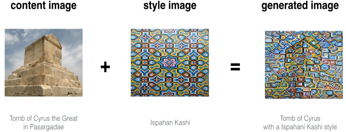
A scientific study of a turbulent fluid with the style of a abstract blue fluid painting.

5 - Test with your own image (Optional/Ungraded)

Finally, you can also rerun the algorithm on your own images!

To do so, go back to part 4 and change the content image and style image with your own pictures. In detail, here's what you should do:

Click on "File -> Open" in the upper tab of the notebook
Go to "/images" and upload your images (requirement: (WIDTH = 400, HEIGHT = 300,像素400*300)), rename them "my_content.png" and "my_style.png" for example.

Change the code in part (3.4) from :

content_image = scipy.misc.imread("images/louvre.jpg")
style_image = scipy.misc.imread("images/claude-monet.jpg")

to:

content_image = scipy.misc.imread("images/my_content.jpg")
style_image = scipy.misc.imread("images/my_style.jpg")

Rerun the cells (you may need to restart the Kernel in the upper tab of the notebook).

You can also tune your hyperparameters:

Which layers are responsible for representing the style? STYLE_LAYERS
How many iterations do you want to run the algorithm? num_iterations
What is the relative weighting between content and style? alpha/beta

6 - Conclusion

Great job on completing this assignment! You are now able to use Neural Style Transfer to generate artistic images. This is also your first time building a model in which the optimization algorithm updates the pixel values rather than the neural network's parameters. Deep learning has many different types of models and this is only one of them!

What you should remember:

Neural Style Transfer is an algorithm that given a content image C and a style image S can generate an artistic image
It uses representations (hidden layer activations) based on a pretrained ConvNet.
The content cost function is computed using one hidden layer's activations.
The style cost function for one layer is computed using the Gram matrix of that layer's activations. The overall style cost function is obtained using several hidden layers.
Optimizing the total cost function results in synthesizing new images.

This was the final programming exercise of this course. Congratulations--you've finished all the programming exercises of this course on Convolutional Networks! We hope to also see you in Course 5, on Sequence models!

References:

The Neural Style Transfer algorithm was due to Gatys et al. (2015). Harish Narayanan and Github user "log0" also have highly readable write-ups from which we drew inspiration. The pre-trained network used in this implementation is a VGG network, which is due to Simonyan and Zisserman (2015). Pre-trained weights were from the work of the MathConvNet team.

Leon A. Gatys, Alexander S. Ecker, Matthias Bethge, (2015). A Neural Algorithm of Artistic Style (https://arxiv.org/abs/1508.06576)
Harish Narayanan, Convolutional neural networks for artistic style transfer. https://harishnarayanan.org/writing/artistic-style-transfer/
Log0, TensorFlow Implementation of "A Neural Algorithm of Artistic Style". http://www.chioka.in/tensorflow-implementation-neural-algorithm-of-artistic-style
Karen Simonyan and Andrew Zisserman (2015). Very deep convolutional networks for large-scale image recognition (https://arxiv.org/pdf/1409.1556.pdf)
MatConvNet. http://www.vlfeat.org/matconvnet/pretrained/

课程四(Convolutional Neural Networks)，第四 周（Special applications: Face recognition & Neural style transfer） —— 2.Programming assignments：Art generation with Neural Style Transfer

Deep Learning & Art: Neural Style Transfer

1 - Problem Statement

2 - Transfer Learning

3 - Neural Style Transfer

3.1 - Computing the content cost

3.2 - Computing the style cost

3.2.1 - Style matrix

3.2.2 - Style cost

3.2.3 Style Weights

3.3 - Defining the total cost to optimize

4 - Solving the optimization problem

5 - Test with your own image (Optional/Ungraded)

6 - Conclusion

References:

课程四(Convolutional Neural Networks)，第四周（Special applications: Face recognition & Neural style transfer） —— 2.Programming assignments：Art generation with Neural Style Transfer