课程一(Neural Networks and Deep Learning)，第四周（Deep Neural Networks）——2.Programming Assignments: Building your Deep Neural Network: Step by Step

Building your Deep Neural Network: Step by Step

Welcome to your third programming exercise of the deep learning specialization. You will implement all the building blocks of a neural network and use these building blocks in the next assignment to build a neural network of any architecture you want. By completing this assignment you will:

- Develop an intuition of the over all structure of a neural network.

- Write functions (e.g. forward propagation, backward propagation, logistic loss, etc...) that would help you decompose your code and ease the process of building a neural network.

- Initialize/update parameters according to your desired structure.

This assignment prepares you well for the upcoming assignment. Take your time to complete it and make sure you get the expected outputs when working through the different exercises. In some code blocks, you will find a "#GRADED FUNCTION: functionName" comment. Please do not modify it. After you are done, submit your work and check your results. You need to score 70% to pass. Good luck :) !

【中文翻译】

一步一步地构建您的深层神经网络

欢迎您来到深度学习专业的第三次编程练习。您将实现神经网络的所有构建块, 并在下一个任务中使用这些构造块来构建您想要的任何体系结构的神经网络。通过完成此任务, 您将:

（1）形成一个神经网络的所有结构的直觉。

 （2）写函数 (如前向传播、反向传播、逻辑损失函数等), 可以帮助您分解代码并简化构建神经网络的过程。

 （3）根据所需的结构初始化/更新参数。

这个任务为即将到来的任务做好准备。用你的时间完成它, 完成不同的练习并确保你得到预期的结果 。在某些代码块中, 您将找到一个"#GRADED FUNCTION: functionName" 的注释。请不要修改它。完成后, 提交您的工作, 并检查您的结果。你需要得分70% 才能过关。祝你好运:)!

--------------------------------------------------------------------------------------------------------------------

Building your Deep Neural Network: Step by Step

Welcome to your week 4 assignment (part 1 of 2)! You have previously trained a 2-layer Neural Network (with a single hidden layer). This week, you will build a deep neural network, with as many layers as you want!

• In this notebook, you will implement all the functions required to build a deep neural network.
• In the next assignment, you will use these functions to build a deep neural network for image classification.

After this assignment you will be able to:

• Use non-linear units like ReLU to improve your model
• Build a deeper neural network (with more than 1 hidden layer)
• Implement an easy-to-use neural network class

Notation:

• Superscript [l] denotes a quantity associated with the l^th layer.
  • Example: a^[L] is the L^th layer activation. W^[L]and b^[L]are the L^th layer parameters.
• Superscript (i) denotes a quantity associated with the i^th example.
  • Example: x⁽ⁱ⁾ is the i^th training example.
• Lowerscript i denotes the i^th entry（项） of a vector.
  • Example: a_i^[l]denotes the i^th entry of the l^th layer's activations.

Let's get started!

1 - Packages

Let's first import all the packages that you will need during this assignment.

• numpy is the main package for scientific computing with Python.
• matplotlib is a library to plot graphs in Python.
• dnn_utils provides some necessary functions for this notebook.
• testCases provides some test cases to assess the correctness of your functions
• np.random.seed(1) is used to keep all the random function calls consistent. It will help us grade your work. Please don't change the seed.

import numpy as np
import h5py
import matplotlib.pyplot as plt
from testCases_v3 import *
from dnn_utils_v2 import sigmoid, sigmoid_backward, relu, relu_backward

%matplotlib inline  # matplotlib inline是jupyter notebook里的命令, 意思是将那些用matplotlib绘制的图显示在页面里而不是弹出一个窗口
plt.rcParams['figure.figsize'] = (5.0, 4.0) # set default size of plots
plt.rcParams['image.interpolation'] = 'nearest'
plt.rcParams['image.cmap'] = 'gray'

%load_ext autoreload   # 在执行用户代码前，重新装入软件的扩展和模块
%autoreload 2 

np.random.seed(1)

 ------------------------------------------------------------------------------------------------------------------

2 - Outline of the Assignment

To build your neural network, you will be implementing several "helper functions". These helper functions will be used in the next assignment to build a two-layer neural network and an L-layer neural network. Each small helper function you will implement will have detailed instructions that will walk you through the necessary steps. Here is an outline of this assignment, you will:

• Initialize the parameters for a two-layer network and for an LL-layer neural network.
• Implement the forward propagation module (shown in purple in the figure below).
  • Complete the LINEAR part of a layer's forward propagation step (resulting in Z[l]Z[l]).
  • We give you the ACTIVATION function (relu/sigmoid).
  • Combine the previous two steps into a new [LINEAR->ACTIVATION] forward function.
  • Stack the [LINEAR->RELU] forward function L-1 time (for layers 1 through L-1) and add a [LINEAR->SIGMOID] at the end (for the final layer LL). This gives you a new L_model_forward function.
• Compute the loss.
• Implement the backward propagation module (denoted in red in the figure below).
  • Complete the LINEAR part of a layer's backward propagation step.
  • We give you the gradient of the ACTIVATE function (relu_backward/sigmoid_backward)
  • Combine the previous two steps into a new [LINEAR->ACTIVATION] backward function.
  • Stack [LINEAR->RELU] backward L-1 times and add [LINEAR->SIGMOID] backward in a new L_model_backward function
• Finally update the parameters.

Note that for every forward function, there is a corresponding backward function. That is why at every step of your forward module you will be storing some values in a cache. The cached values are useful for computing gradients. In the backpropagation module you will then use the cache to calculate the gradients. This assignment will show you exactly how to carry out each of these steps.

【中文翻译】

2-任务的概要

　　为了建立你的神经网络, 你将实现几个 "帮助函数"。这些帮助函数将用于下一个任务, 以构建一个双层神经网络和一个 L层神经网络。您将实现的每个小帮手功能将有详细的说明, 将指导您完成必要的步骤。下面是此任务的大纲, 您将:

　　1）初始化两层网络和 L 层神经网络的参数。

　　2）实现正向传播模块 (以紫色显示在下图中)。

　　　　（1）完成层的正向传播步骤的线性部分 (导致 Z^[l])。

　　　　（2）我们给你的激活函数 (relu/sigmoid)。

　　　　（3）将前两个步骤合并为一个新的 [LINEAR->ACTIVATION] 前向传播函数。

　　　　（4）堆叠 [LINEAR->RELU]前向传播函数 L-1 次 (从第1层到 L-1层) 和添加一个 [LINEAR->SIGMOID] 在最后(最后一层 L)。这为您提供了一个新的 L_model_forward 函数。

　　3）计算损失。

　　4）实现向后传播模块 (在下图中用红色表示)。

　　　　（1）完成后向传播步骤的线性部分。

　　　　（2）我们给你的激活函数的梯度 (relu_backward/sigmoid_backward)

　　　　（3）将前两个步骤合并为一个新的 [[LINEAR->ACTIVATION] 向后传播函数。

　　　　（4）叠加 [LINEAR->RELU] 向后 L-1 次，并在新的 L_model_backward 函数中向后添加 [LINEAR->SIGMOID]

　　5）最后更新参数。

 

 ------------------------------------------------------------------------------------------------------------------

3 - Initialization

You will write two helper functions that will initialize the parameters for your model. The first function will be used to initialize parameters for a two layer model. The second one will generalize this initialization process to LL layers.

【中文翻译】

您将编写两个帮助函数来初始化模型的参数。第一个函数将用于初始化两层模型的参数。第二个将把这个初始化过程推广到L 层。

3.1 - 2-layer Neural Network

Exercise: Create and initialize the parameters of the 2-layer neural network.

Instructions:

• The model's structure is: LINEAR -> RELU -> LINEAR -> SIGMOID.
• Use random initialization for the weight matrices. Use np.random.randn(shape)*0.01 with the correct shape.
• Use zero initialization for the biases. Use np.zeros(shape).

【code】

# GRADED FUNCTION: initialize_parameters

def initialize_parameters(n_x, n_h, n_y):
    """
    Argument:
    n_x -- size of the input layer
    n_h -- size of the hidden layer
    n_y -- size of the output layer
    
    Returns:
    parameters -- python dictionary containing your parameters:
                    W1 -- weight matrix of shape (n_h, n_x)
                    b1 -- bias vector of shape (n_h, 1)
                    W2 -- weight matrix of shape (n_y, n_h)
                    b2 -- bias vector of shape (n_y, 1)
    """
    
    np.random.seed(1)
    
    ### START CODE HERE ### (≈ 4 lines of code)
    W1 = np.random.randn(n_h, n_x)*0.01
    b1 = np.zeros((n_h, 1))
    W2 = np.random.randn(n_y, n_h)*0.01
    b2 = np.zeros((n_y, 1))
    ### END CODE HERE ###
    
    assert(W1.shape == (n_h, n_x))
    assert(b1.shape == (n_h, 1))
    assert(W2.shape == (n_y, n_h))
    assert(b2.shape == (n_y, 1))
    
    parameters = {"W1": W1,
                  "b1": b1,
                  "W2": W2,
                  "b2": b2}
    
    return parameters    

parameters = initialize_parameters(3,2,1)
print("W1 = " + str(parameters["W1"]))
print("b1 = " + str(parameters["b1"]))
print("W2 = " + str(parameters["W2"]))
print("b2 = " + str(parameters["b2"]))

【result】

W1 = [[ 0.01624345 -0.00611756 -0.00528172]
 [-0.01072969  0.00865408 -0.02301539]]
b1 = [[ 0.]
 [ 0.]]
W2 = [[ 0.01744812 -0.00761207]]
b2 = [[ 0.]]

Expected output:

W1	[[ 0.01624345 -0.00611756 -0.00528172] [-0.01072969 0.00865408 -0.02301539]]
b1	[[ 0.] [ 0.]]
W2	[[ 0.01744812 -0.00761207]]
b2	[[ 0.]]

3.2 - L-layer Neural Network

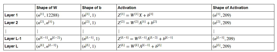
The initialization for a deeper L-layer neural network is more complicated because there are many more weight matrices and bias vectors. When completing the initialize_parameters_deep, you should make sure that your dimensions match between each layer. Recall that n[l]n[l] is the number of units in layer ll.

Thus for example if the size of our input XX is (12288,209)(12288,209) (with m=209m=209 examples) then:

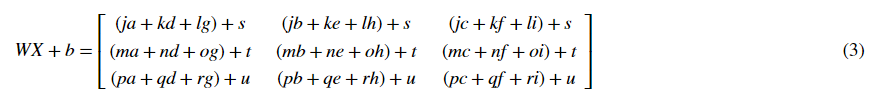
Remember that when we compute WX+bWX+b in python, it carries out broadcasting. For example, if:

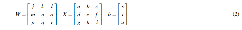
Then WX+b will be:

Exercise: Implement initialization for an L-layer Neural Network.

Instructions:

• The model's structure is [LINEAR -> RELU] ×× (L-1) -> LINEAR -> SIGMOID. I.e., it has L−1L−1 layers using a ReLU activation function followed by an output layer with a sigmoid activation function.
• Use random initialization for the weight matrices. Use np.random.rand(shape) * 0.01.
• Use zeros initialization for the biases. Use np.zeros(shape).
• We will store n[l]n[l], the number of units in different layers, in a variable layer_dims. For example, the layer_dims for the "Planar Data classification model" from last week would have been [2,4,1]: There were two inputs, one hidden layer with 4 hidden units, and an output layer with 1 output unit. Thus means W1's shape was (4,2), b1 was (4,1), W2 was (1,4) and b2 was (1,1). Now you will generalize this to LL layers!
• Here is the implementation for L=1L=1 (one layer neural network). It should inspire you to implement the general case (L-layer neural network).

    if L == 1:
        parameters["W" + str(L)] = np.random.randn(layer_dims[1], layer_dims[0]) * 0.01
        parameters["b" + str(L)] = np.zeros((layer_dims[1], 1))

【code】

# GRADED FUNCTION: initialize_parameters_deep

def initialize_parameters_deep(layer_dims):
    """
    Arguments:
    layer_dims -- python array (list) containing the dimensions of each layer in our network
    
    Returns:
    parameters -- python dictionary containing your parameters "W1", "b1", ..., "WL", "bL":
                    Wl -- weight matrix of shape (layer_dims[l], layer_dims[l-1])
                    bl -- bias vector of shape (layer_dims[l], 1)
    """
    
    np.random.seed(3)
    parameters = {}
    L = len(layer_dims)            # number of layers in the network

    for l in range(1, L):
        ### START CODE HERE ### (≈ 2 lines of code)
        parameters['W' + str(l)] =  np.random.randn(layer_dims[l], layer_dims[l-1]) * 0.01
        parameters['b' + str(l)] =  np.zeros((layer_dims[l], 1))
        ### END CODE HERE ###
        
        assert(parameters['W' + str(l)].shape == (layer_dims[l], layer_dims[l-1]))
        assert(parameters['b' + str(l)].shape == (layer_dims[l], 1))

        
    return parameters

parameters = initialize_parameters_deep([5,4,3])
print("W1 = " + str(parameters["W1"]))
print("b1 = " + str(parameters["b1"]))
print("W2 = " + str(parameters["W2"]))
print("b2 = " + str(parameters["b2"]))

【result】

W1 = [[ 0.01788628  0.0043651   0.00096497 -0.01863493 -0.00277388]
 [-0.00354759 -0.00082741 -0.00627001 -0.00043818 -0.00477218]
 [-0.01313865  0.00884622  0.00881318  0.01709573  0.00050034]
 [-0.00404677 -0.0054536  -0.01546477  0.00982367 -0.01101068]]
b1 = [[ 0.]
 [ 0.]
 [ 0.]
 [ 0.]]
W2 = [[-0.01185047 -0.0020565   0.01486148  0.00236716]
 [-0.01023785 -0.00712993  0.00625245 -0.00160513]
 [-0.00768836 -0.00230031  0.00745056  0.01976111]]
b2 = [[ 0.]
 [ 0.]
 [ 0.]]

Expected output:

W1	[[ 0.01788628 0.0043651 0.00096497 -0.01863493 -0.00277388] [-0.00354759 -0.00082741 -0.00627001 -0.00043818 -0.00477218] [-0.01313865 0.00884622 0.00881318 0.01709573 0.00050034] [-0.00404677 -0.0054536 -0.01546477 0.00982367 -0.01101068]]
b1	[[ 0.] [ 0.] [ 0.] [ 0.]]
W2	[[-0.01185047 -0.0020565 0.01486148 0.00236716] [-0.01023785 -0.00712993 0.00625245 -0.00160513] [-0.00768836 -0.00230031 0.00745056 0.01976111]]
b2	[[ 0.] [ 0.] [ 0.]]

 

 ------------------------------------------------------------------------------------------------------------------------------------------------------------

4 - Forward propagation module

4.1 - Linear Forward

Now that you have initialized your parameters, you will do the forward propagation module. You will start by implementing some basic functions that you will use later when implementing the model. You will complete three functions in this order:

• LINEAR
• LINEAR -> ACTIVATION where ACTIVATION will be either ReLU or Sigmoid.
• [LINEAR -> RELU] × (L-1) -> LINEAR -> SIGMOID (whole model)

The linear forward module (vectorized over all the examples) computes the following equations:

where A^[0]=X.

Exercise: Build the linear part of forward propagation.

Reminder: The mathematical representation of this unit is Z^[l]=W^[l]A^[l−1]+b^[l]. You may also find np.dot() useful. If your dimensions don't match, printing W.shape may help.

【code】

# GRADED FUNCTION: linear_forward

def linear_forward(A, W, b):
    """
    Implement the linear part of a layer's forward propagation.

    Arguments:
    A -- activations from previous layer (or input data): (size of previous layer, number of examples)
    W -- weights matrix: numpy array of shape (size of current layer, size of previous layer)
    b -- bias vector, numpy array of shape (size of the current layer, 1)

    Returns:
    Z -- the input of the activation function, also called pre-activation parameter 
    cache -- a python dictionary containing "A", "W" and "b" ; stored for computing the backward pass efficiently
    """
    
    ### START CODE HERE ### (≈ 1 line of code)
    Z = np.dot(W,A)+b
    ### END CODE HERE ###
    
    assert(Z.shape == (W.shape[0], A.shape[1])) # W的行数，Z的列数
    cache = (A, W, b)
    
    return Z, cache

A, W, b = linear_forward_test_case()

Z, linear_cache = linear_forward(A, W, b)
print("Z = " + str(Z))

【result】

Z = [[ 3.26295337 -1.23429987]]

Expected output:

Z	[[ 3.26295337 -1.23429987]]

4.2 - Linear-Activation Forward

In this notebook, you will use two activation functions:

• Sigmoid: 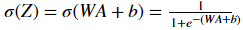. We have provided you with the sigmoid function. This function returns two items: the activation value "a" and a "cache" that contains "Z" (it's what we will feed in to the corresponding backward function). To use it you could just call:

  A, activation_cache = sigmoid(Z)
  

• ReLU: The mathematical formula for ReLu is We have provided you with the relu function. This function returns two items: the activation value "A" and a "cache" that contains "Z" (it's what we will feed in to the corresponding backward function). To use it you could just call:

  A, activation_cache = relu(Z)

For more convenience, you are going to group two functions (Linear and Activation) into one function (LINEAR->ACTIVATION). Hence, you will implement a function that does the LINEAR forward step followed by an ACTIVATION forward step.

Exercise: Implement the forward propagation of the LINEAR->ACTIVATION layer. Mathematical relation is: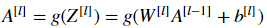 where the activation "g" can be sigmoid() or relu(). Use linear_forward() and the correct activation function.

【中文翻译】

4.2-向前传播的线性+激活函数

在本笔记本中, 您将使用两个激活函数:

Sigmoid: ，我们为您提供了 sigmoid（） 函数。此函数返回两个项: 激活值 "a" 和包含 "Z" 的 "缓存" (Z是我们在相应的反向传播函数中输入的内容)。要使用它, 您可以只调用:

 　　A, activation_cache = sigmoid(Z)

ReLU: ReLU 的数学公式是 此函数返回两个项: 激活值 "a" 和包含 "Z" 的 "缓存" (Z是我们在相应的反向传播函数中输入的内容)。要使用它, 您可以只调用:

   A, activation_cache = relu(Z)

为了更方便起见, 您要将两个函数 (线性和激活) 合为一个函数 (线性+激活函数)。因此, 您将实现一个函数, 它执行线性向前步骤, 后跟一个激活向前步骤。

练习: 实现线性--->激活层的正向传播。数学关系是:。 激活函数 "g" 可以是sigmoid() or relu()。

使用 linear_forward () 和正确的激活函数。

【code】 

# GRADED FUNCTION: linear_activation_forward

def linear_activation_forward(A_prev, W, b, activation):
    """
    Implement the forward propagation for the LINEAR->ACTIVATION layer

    Arguments:
    A_prev -- activations from previous layer (or input data): (size of previous layer, number of examples)
    W -- weights matrix: numpy array of shape (size of current layer, size of previous layer)
    b -- bias vector, numpy array of shape (size of the current layer, 1)
    activation -- the activation to be used in this layer, stored as a text string: "sigmoid" or "relu"

    Returns:
    A -- the output of the activation function, also called the post-activation value（后面的值） 
    cache -- a python dictionary containing "linear_cache" and "activation_cache";
             stored for computing the backward pass efficiently
    """
    
    if activation == "sigmoid":
        # Inputs: "A_prev, W, b". Outputs: "A, activation_cache".
        ### START CODE HERE ### (≈ 2 lines of code)
        Z, linear_cache =  linear_forward(A_prev, W, b)
        A, activation_cache = sigmoid(Z)
        ### END CODE HERE ###
    
    elif activation == "relu":
        # Inputs: "A_prev, W, b". Outputs: "A, activation_cache".
        ### START CODE HERE ### (≈ 2 lines of code)
        Z, linear_cache =linear_forward(A_prev, W, b)
        A, activation_cache = relu(Z)
        ### END CODE HERE ###
    
    assert (A.shape == (W.shape[0], A_prev.shape[1]))
    cache = (linear_cache, activation_cache)

    return A, cache

A_prev, W, b = linear_activation_forward_test_case()

A, linear_activation_cache = linear_activation_forward(A_prev, W, b, activation = "sigmoid")
print("With sigmoid: A = " + str(A))

A, linear_activation_cache = linear_activation_forward(A_prev, W, b, activation = "relu")
print("With ReLU: A = " + str(A))

 【result】

With sigmoid: A = [[ 0.96890023  0.11013289]]
With ReLU: A = [[ 3.43896131  0.        ]]

Expected output:

With sigmoid: A	[[ 0.96890023 0.11013289]]
With ReLU: A	[[ 3.43896131 0. ]]

Note: In deep learning, the "[LINEAR->ACTIVATION]" computation is counted as a single layer in the neural network, not two layers.

 

4.3 L-Layer Model

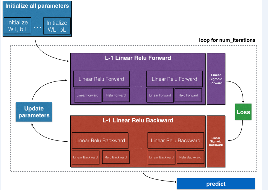
For even more convenience when implementing the L-layer Neural Net, you will need a function that replicates the previous one (linear_activation_forward with RELU) L−1 times, then follows that with one linear_activation_forward with SIGMOID.

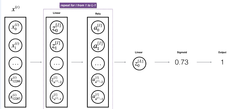
　　　　Figure 2 : [LINEAR -> RELU] × (L-1) -> LINEAR -> SIGMOID model

Exercise: Implement the forward propagation of the above model.

Instruction: In the code below, the variable AL will denote 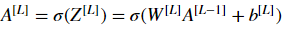. (This is sometimes also called Yhat, i.e., this is )

Tips:

• Use the functions you had previously written
• Use a for loop to replicate [LINEAR->RELU] (L-1) times
• Don't forget to keep track of the caches in the "caches" list. To add a new value c to a list, you can use list.append(c).

 

 【Tips中文翻译】

提示:

　　使用以前编写的函数

　　使用 for 循环复制  [LINEAR->RELU] (L-1)次

　　不要忘记在 "缓存" 列表中记录缓存。若要向list中添加新的值 c, 可以使用 list.append(c).

 【code】

# GRADED FUNCTION: L_model_forward

def L_model_forward(X, parameters):
    """
    Implement forward propagation for the [LINEAR->RELU]*(L-1)->LINEAR->SIGMOID computation
    
    Arguments:
    X -- data, numpy array of shape (input size, number of examples)
    parameters -- output of initialize_parameters_deep()
    
    Returns:
    AL -- last post-activation value
    caches -- list of caches containing:
                every cache of linear_relu_forward() (there are L-1 of them, indexed from 0 to L-2)
                the cache of linear_sigmoid_forward() (there is one, indexed L-1)
    """

    caches = []
    A = X
    L = len(parameters) // 2       # number of layers in the neural network
    
    # Implement [LINEAR -> RELU]*(L-1). Add "cache" to the "caches" list.
    for l in range(1, L):   #注意range是(1,L),最后的L不算进循环
        A_prev = A 
        ### START CODE HERE ### (≈ 2 lines of code)
        A, cache = linear_activation_forward(A_prev, parameters['W'+str(l)], parameters['b'+str(l)], activation = "relu")
        caches.append(cache)
        ### END CODE HERE ###
    
    # Implement LINEAR -> SIGMOID. Add "cache" to the "caches" list.
    ### START CODE HERE ### (≈ 2 lines of code)
    AL, cache = linear_activation_forward(A, parameters['W'+str(L)], parameters['b'+str(L)], activation = "sigmoid")
    caches.append(cache) 
    ### END CODE HERE ###
    
    assert(AL.shape == (1,X.shape[1]))
            
    return AL, caches

X, parameters = L_model_forward_test_case_2hidden()
AL, caches = L_model_forward(X, parameters)
print("AL = " + str(AL))
print("Length of caches list = " + str(len(caches)))

【result】

AL = [[ 0.03921668  0.70498921  0.19734387  0.04728177]]
Length of caches list = 3

Expected output:

AL	[[ 0.03921668 0.70498921 0.19734387 0.04728177]]
Length of caches list	3

Great! Now you have a full forward propagation that takes the input X and outputs a row vector A[L]A[L] containing your predictions. It also records

all intermediate values in "caches". Using A[L]A[L], you can compute the cost of your predictions.　　

----------------------------------------------------------------------------------------------

5 - Cost function

Now you will implement forward and backward propagation. You need to compute the cost, because you want to check if your model is actually learning.

Exercise: Compute the cross-entropy cost J （交叉熵成本函数J）, using the following formula:

【code】

# GRADED FUNCTION: compute_cost

def compute_cost(AL, Y):
    """
    Implement the cost function defined by equation (7).

    Arguments:
    AL -- probability vector corresponding to your label predictions, shape (1, number of examples)
    Y -- true "label" vector (for example: containing 0 if non-cat, 1 if cat), shape (1, number of examples)

    Returns:
    cost -- cross-entropy cost
    """
    
    m = Y.shape[1]

    # Compute loss from aL and y.
    ### START CODE HERE ### (≈ 1 lines of code)
    cost = - (np.dot(Y, np.log(AL).T) + np.dot(1 - Y,np.log(1-AL).T)) / m
    ### END CODE HERE ###
    
    cost = np.squeeze(cost)      # To make sure your cost's shape is what we expect (e.g. this turns [[17]] into 17).
    assert(cost.shape == ())
    
    return cost

Y, AL = compute_cost_test_case()

print("cost = " + str(compute_cost(AL, Y)))

【result】

cost = 0.414931599615397

Expected Output:

cost	0.41493159961539694

-----------------------------------------------------------------------------------------------------------

6 - Backward propagation module

Just like with forward propagation, you will implement helper functions for backpropagation. Remember that back propagation is used to calculate

the gradient of the loss function with respect to the parameters.

Reminder:

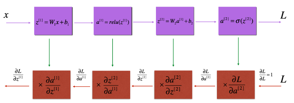
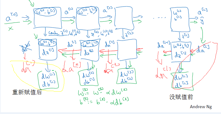
              Figure 3 : Forward and Backward propagation for LINEAR->RELU->LINEAR->SIGMOID 

The purple blocks represent the forward propagation, and the red blocks represent the backward propagation.

Now, similar to forward propagation, you are going to build the backward propagation in three steps:

• LINEAR backward
• LINEAR -> ACTIVATION backward where ACTIVATION computes the derivative of either the ReLU or sigmoid activation
• [LINEAR -> RELU] ×× (L-1) -> LINEAR -> SIGMOID backward (whole model)

6.1 - Linear backward

For layer ll, the linear part is: 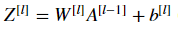 (followed by an activation).

Suppose you have already calculated the derivative 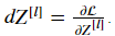 You want to get  (dW^[l],db^[l],dA^[l]) 

       

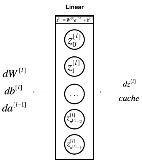
                                     Figure 4

The three outputs (dW^[l],db^[l],dA^[l-1]) are computed using the input dZ^[l] Here are the formulas you need:

 

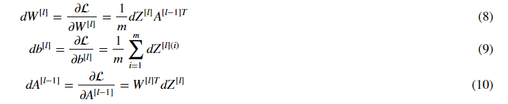
Exercise: Use the 3 formulas above to implement linear_backward().

【code】

# GRADED FUNCTION: linear_backward

def linear_backward(dZ, cache):
    """
    Implement the linear portion of backward propagation for a single layer (layer l)

    Arguments:
    dZ -- Gradient of the cost with respect to the linear output (of current layer l)
    cache -- tuple of values (A_prev, W, b) coming from the forward propagation in the current layer

    Returns:
    dA_prev -- Gradient of the cost with respect to the activation (of the previous layer l-1), same shape as A_prev
    dW -- Gradient of the cost with respect to W (current layer l), same shape as W
    db -- Gradient of the cost with respect to b (current layer l), same shape as b
    """
    A_prev, W, b = cache
    m = A_prev.shape[1]

    ### START CODE HERE ### (≈ 3 lines of code)
    dW = np.dot(dZ, A_prev.T)/m
    db = np.sum(dZ,axis=1,keepdims=True)/m   # 按照行相加,axis=1
    dA_prev = np.dot(W.T, dZ)
    ### END CODE HERE ###
    
    assert (dA_prev.shape == A_prev.shape)
    assert (dW.shape == W.shape)
    assert (db.shape == b.shape)
    
    return dA_prev, dW, db

# Set up some test inputs
dZ, linear_cache = linear_backward_test_case()

dA_prev, dW, db = linear_backward(dZ, linear_cache)    
print ("dA_prev = "+ str(dA_prev))
print ("dW = " + str(dW))
print ("db = " + str(db))

【result】

dA_prev = [[ 0.51822968 -0.19517421]
 [-0.40506361  0.15255393]
 [ 2.37496825 -0.89445391]]
dW = [[-0.10076895  1.40685096  1.64992505]]
db = [[ 0.50629448]]

Expected Output:

dA_prev	[[ 0.51822968 -0.19517421] [-0.40506361 0.15255393] [ 2.37496825 -0.89445391]]
dW	[[-0.10076895 1.40685096 1.64992505]]
db	[[ 0.50629448]]

 

6.2 - Linear-Activation backward

Next, you will create a function that merges the two helper functions: linear_backward and the backward step for the activation linear_activation_backward.

To help you implement linear_activation_backward, we provided two backward functions:

• sigmoid_backward: Implements the backward propagation for SIGMOID unit. You can call it as follows:

dZ = sigmoid_backward(dA, activation_cache)

• relu_backward: Implements the backward propagation for RELU unit. You can call it as follows:

dZ = relu_backward(dA, activation_cache)

If g(.) is the activation function, sigmoid_backward and relu_backward compute

【中文翻译】

接下来, 您将创建一个合并两个 helper 函数的函数: linear_backward 和激活 linear_activation_backward 的向后步骤。

为了帮助您实现 linear_activation_backward, 我们提供了两个向后的函数:

　　sigmoid_backward: 实现对 SIGMOID单元的反向传播。您可以按如下所示调用它:

　　　　dZ = sigmoid_backward (dA, activation_cache)

　　relu_backward: 实现 relu 单元的反向传播。您可以按如下所示调用它:

　　　　dZ = relu_backward (dA, activation_cache)

如果 g (.) 是激活函数, sigmoid_backward 和 relu_backward 计算

.

 【code】

# GRADED FUNCTION: linear_activation_backward

def linear_activation_backward(dA, cache, activation):
    """
    Implement the backward propagation for the LINEAR->ACTIVATION layer.
    
    Arguments:
    dA -- post-activation gradient for current layer l 
    cache -- tuple of values (linear_cache, activation_cache) we store for computing backward propagation efficiently
    activation -- the activation to be used in this layer, stored as a text string: "sigmoid" or "relu"
    
    Returns:
    dA_prev -- Gradient of the cost with respect to the activation (of the previous layer l-1), same shape as A_prev
    dW -- Gradient of the cost with respect to W (current layer l), same shape as W
    db -- Gradient of the cost with respect to b (current layer l), same shape as b
    """
    linear_cache, activation_cache = cache
    
    if activation == "relu":  
        ### START CODE HERE ### (≈ 2 lines of code)           # ??? 什么是activation_cache
        dZ = relu_backward(dA, activation_cache) 
        dA_prev, dW, db = linear_backward(dZ, linear_cache)    # ??? 什么是linear_cache
        ### END CODE HERE ###
        
    elif activation == "sigmoid":
        ### START CODE HERE ### (≈ 2 lines of code)
        dZ = sigmoid_backward(dA, activation_cache)           
        dA_prev, dW, db = linear_backward(dZ, linear_cache)
        ### END CODE HERE ###
    
    return dA_prev, dW, db

dA, linear_activation_cache = linear_activation_backward_test_case()

dA_prev, dW, db = linear_activation_backward(dA, linear_activation_cache, activation = "sigmoid")
print ("sigmoid:")
print ("dA_prev = "+ str(dA_prev))
print ("dW = " + str(dW))
print ("db = " + str(db) + " ")

dA_prev, dW, db = linear_activation_backward(dA, linear_activation_cache, activation = "relu")
print ("relu:")
print ("dA_prev = "+ str(dA_prev))
print ("dW = " + str(dW))
print ("db = " + str(db))

【result】

sigmoid:
dA_prev = [[ 0.11017994  0.01105339]
 [ 0.09466817  0.00949723]
 [-0.05743092 -0.00576154]]
dW = [[ 0.10266786  0.09778551 -0.01968084]]
db = [[-0.05729622]]

relu:
dA_prev = [[ 0.44090989  0.        ]
 [ 0.37883606  0.        ]
 [-0.2298228   0.        ]]
dW = [[ 0.44513824  0.37371418 -0.10478989]]
db = [[-0.20837892]]

Expected output with sigmoid:

dA_prev	[[ 0.11017994 0.01105339] [ 0.09466817 0.00949723] [-0.05743092 -0.00576154]]
dW	[[ 0.10266786 0.09778551 -0.01968084]]
db	[[-0.05729622]]

Expected output with relu:

dA_prev	[[ 0.44090989 0. ] [ 0.37883606 0. ] [-0.2298228 0. ]]
dW	[[ 0.44513824 0.37371418 -0.10478989]]
db	[[-0.20837892]]

6.3 - L-Model Backward

Now you will implement the backward function for the whole network. Recall that when you implemented the L_model_forwardfunction, at each iteration, you stored a cache which contains (X,W,b, and z). In the back propagation module, you will use those variables to compute the gradients. Therefore, in the L_model_backward function, you will iterate through all the hidden layers backward, starting from layer LL. On each step, you will use the cached values for layer ll to backpropagate through layer ll. Figure 5 below shows the backward pass.

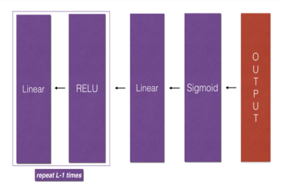
                                      Figure 5 : Backward pass

Initializing backpropagation: To backpropagate through this network, we know that the output is, A[L]=σ(Z[L])A[L]=σ(Z[L]). Your code thus needs to compute 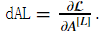To do so, use this formula (derived using calculus which you don't need in-depth knowledge of)

dAL = - (np.divide(Y, AL) - np.divide(1 - Y, 1 - AL)) # derivative of cost with respect to AL

You can then use this post-activation gradient dAL to keep going backward. As seen in Figure 5, you can now feed in dAL into the LINEAR->SIGMOID backward function you implemented (which will use the cached values stored by the L_model_forward function). After that, you will have to use a for loop to iterate through all the other layers using the LINEAR->RELU backward function. You should store each dA, dW, and db in the grads dictionary. To do so, use this formula :

　　　　　　　　grads["dW"+str(l)]=dW^[l]                                                    (15)

For example, for l=3l=3 this would store dW^[l] in grads["dW3"].

Exercise: Implement backpropagation for the [LINEAR->RELU] × (L-1) -> LINEAR -> SIGMOID model.

【code】

# GRADED FUNCTION: L_model_backward

def L_model_backward(AL, Y, caches):
    """
    Implement the backward propagation for the [LINEAR->RELU] * (L-1) -> LINEAR -> SIGMOID group
    
    Arguments:
    AL -- probability vector, output of the forward propagation (L_model_forward())
    Y -- true "label" vector (containing 0 if non-cat, 1 if cat)
    caches -- list of caches containing:
                every cache of linear_activation_forward() with "relu" (it's caches[l], for l in range(L-1) i.e l = 0...L-2)
                the cache of linear_activation_forward() with "sigmoid" (it's caches[L-1])
    
    Returns:
    grads -- A dictionary with the gradients
             grads["dA" + str(l)] = ... 
             grads["dW" + str(l)] = ...
             grads["db" + str(l)] = ... 
    """
    grads = {}
    L = len(caches) # the number of layers
    m = AL.shape[1]
    Y = Y.reshape(AL.shape) # after this line, Y is the same shape as AL
    
    # Initializing the backpropagation
    ### START CODE HERE ### (1 line of code)
    dAL = - (np.divide(Y, AL) - np.divide(1 - Y, 1 - AL)) # derivative of cost with respect to AL
    ### END CODE HERE ###
    
    # Lth layer (SIGMOID -> LINEAR) gradients. Inputs: "AL, Y, caches". Outputs: "grads["dAL"], grads["dWL"], grads["dbL"]
    ### START CODE HERE ### (approx. 2 lines)
    current_cache = caches[L-1]
    grads["dA" + str(L)], grads["dW" + str(L)], grads["db" + str(L)] =linear_activation_backward(dAL, current_cache, activation = "sigmoid")  
    ### 上面的函数linear_activation_backward（...）的得到的第一个参数应该是grads["dA" + str(L-1)]，此处把该值赋给grads["dA" + str(L) ，详细见下面的解释图

    ### END CODE HERE ###
    
    for l in reversed(range(L-1)):
        # lth layer: (RELU -> LINEAR) gradients.
        # Inputs: "grads["dA" + str(l + 2)], caches". Outputs: "grads["dA" + str(l + 1)] , grads["dW" + str(l + 1)] , grads["db" + str(l + 1)] 
        ### START CODE HERE ### (approx. 5 lines)
        current_cache =  caches[l]    # L-2,L-1,...,2,1,0   当l=L-2时
        dA_prev_temp, dW_temp, db_temp = linear_activation_backward(grads["dA" + str(l+2)], current_cache, activation = "relu")  # l+2=L
        grads["dA" + str(l + 1)] = dA_prev_temp     #l+1=L-1
        grads["dW" + str(l + 1)] = dW_temp      #l+1=L-1
        grads["db" + str(l + 1)] = db_temp      #l+1=L-1
        ### END CODE HERE ###

    return grads

 【解释】

 

【code】

AL, Y_assess, caches = L_model_backward_test_case()
grads = L_model_backward(AL, Y_assess, caches)
print_grads(grads)

【result】

dW1 = [[ 0.41010002  0.07807203  0.13798444  0.10502167]
 [ 0.          0.          0.          0.        ]
 [ 0.05283652  0.01005865  0.01777766  0.0135308 ]]
db1 = [[-0.22007063]
 [ 0.        ]
 [-0.02835349]]
dA1 = [[ 0.12913162 -0.44014127]
 [-0.14175655  0.48317296]
 [ 0.01663708 -0.05670698]]

Expected Output

dW1	[[ 0.41010002 0.07807203 0.13798444 0.10502167] [ 0. 0. 0. 0. ] [ 0.05283652 0.01005865 0.01777766 0.0135308 ]]
db1	[[-0.22007063] [ 0. ] [-0.02835349]]
dA1	[[ 0.12913162 -0.44014127] [-0.14175655 0.48317296] [ 0.01663708 -0.05670698]]

6.4 - Update Parameters

In this section you will update the parameters of the model, using gradient descent:

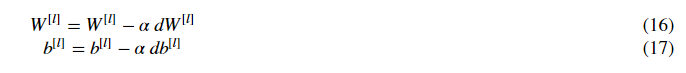
where α is the learning rate. After computing the updated parameters, store them in the parameters dictionary.

Exercise: Implement update_parameters() to update your parameters using gradient descent.

Instructions: Update parameters using gradient descent on every W^[l]and b^[l]for l=1,2,...,l=1,2,...,L.

【code】

# GRADED FUNCTION: update_parameters

def update_parameters(parameters, grads, learning_rate):
    """
    Update parameters using gradient descent
    
    Arguments:
    parameters -- python dictionary containing your parameters 
    grads -- python dictionary containing your gradients, output of L_model_backward
    
    Returns:
    parameters -- python dictionary containing your updated parameters 
                  parameters["W" + str(l)] = ... 
                  parameters["b" + str(l)] = ...
    """
    
    L = len(parameters) // 2 # number of layers in the neural network

    # Update rule for each parameter. Use a for loop.
    ### START CODE HERE ### (≈ 3 lines of code)
    for l in range(1, L+1):   # l=`,2,3,...,L
         parameters["W" + str(l)] = parameters["W" + str(l)] - learning_rate*grads["dW" + str(l)]
         parameters["b" + str(l)] = parameters["b" + str(l)] - learning_rate*grads["db" + str(l)]
    ### END CODE HERE ###
    return parameters

parameters, grads = update_parameters_test_case()
parameters = update_parameters(parameters, grads, 0.1)

print ("W1 = "+ str(parameters["W1"]))
print ("b1 = "+ str(parameters["b1"]))
print ("W2 = "+ str(parameters["W2"]))
print ("b2 = "+ str(parameters["b2"]))

【result】

W1 = [[-0.59562069 -0.09991781 -2.14584584  1.82662008]
 [-1.76569676 -0.80627147  0.51115557 -1.18258802]
 [-1.0535704  -0.86128581  0.68284052  2.20374577]]
b1 = [[-0.04659241]
 [-1.28888275]
 [ 0.53405496]]
W2 = [[-0.55569196  0.0354055   1.32964895]]
b2 = [[-0.84610769]]

Expected Output:

W1	[[-0.59562069 -0.09991781 -2.14584584 1.82662008] [-1.76569676 -0.80627147 0.51115557 -1.18258802] [-1.0535704 -0.86128581 0.68284052 2.20374577]]
b1	[[-0.04659241] [-1.28888275] [ 0.53405496]]
W2	[[-0.55569196 0.0354055 1.32964895]]
b2	[[-0.84610769]]

----------------------------------------------------------------

7 - Conclusion

Congrats on implementing all the functions required for building a deep neural network!

We know it was a long assignment but going forward it will only get better. The next part of the assignment is easier.

In the next assignment you will put all these together to build two models:

• A two-layer neural network
• An L-layer neural network

You will in fact use these models to classify cat vs non-cat images!