Fork版本项目地址:SSD
上一节中我们定义了vgg_300的网络结构,实际使用中还需要匹配SSD另一关键组件:被选取特征层的搜索网格。在项目中,vgg_300网络和网格生成都被统一进一个class中,我们从class SSDNet开始谈起。
一、初始化class SSDNet
这是SSDNet的初始化部分,这一部分的内容在上一节都提到过了:网络超参数定义 & 初始化vgg_300网络结构并更新feat_shapes
【注1】:feat_shapes更新之前每一元素是二维元组(HW),更新之后变成三维(HWC),不影响使用,实际使用时会采取[1:3]切片。
【注2】:虽然给的参数是输入300*300的图片,实际测试中想要匹配后面的feat_shape,需要304*304的输入才行
SSDParams = namedtuple('SSDParameters', ['img_shape',
                                         'num_classes',
                                         'no_annotation_label',
                                         'feat_layers',
                                         'feat_shapes',
                                         'anchor_size_bounds',
                                         'anchor_sizes',
                                         'anchor_ratios',
                                         'anchor_steps',
                                         'anchor_offset',
                                         'normalizations',
                                         'prior_scaling'
                                         ])


class SSDNet(object):
    """Implementation of the SSD VGG-based 300 network.

    The default features layers with 300x300 image input are:
      conv4 ==> 38 x 38
      conv7 ==> 19 x 19
      conv8 ==> 10 x 10
      conv9 ==> 5 x 5
      conv10 ==> 3 x 3
      conv11 ==> 1 x 1
    The default image size used to train this network is 300x300.
    """
    default_params = SSDParams(
        img_shape=(300, 300),
        num_classes=21,
        no_annotation_label=21,
        feat_layers=['block4', 'block7', 'block8', 'block9', 'block10', 'block11'],
        feat_shapes=[(38, 38), (19, 19), (10, 10), (5, 5), (3, 3), (1, 1)],
        anchor_size_bounds=[0.15, 0.90],
        # anchor_size_bounds=[0.20, 0.90],
        anchor_sizes=[(21., 45.),
                      (45., 99.),
                      (99., 153.),
                      (153., 207.),
                      (207., 261.),
                      (261., 315.)],
        anchor_ratios=[[2, .5],
                       [2, .5, 3, 1./3],
                       [2, .5, 3, 1./3],
                       [2, .5, 3, 1./3],
                       [2, .5],
                       [2, .5]],
        anchor_steps=[8, 16, 32, 64, 100, 300],
        anchor_offset=0.5,
        normalizations=[1, -1, -1, -1, -1, -1],  # 控制SSD层处理时是否预先沿着HW正则化
        prior_scaling=[0.1, 0.1, 0.2, 0.2]
        )

    def __init__(self, params=None):
        """Init the SSD net with some parameters. Use the default ones
        if none provided.
        """
        if isinstance(params, SSDParams):
            self.params = params
        else:
            self.params = SSDNet.default_params

    # ======================================================================= #
    def net(self, inputs,
            is_training=True,
            update_feat_shapes=True,
            dropout_keep_prob=0.5,
            prediction_fn=slim.softmax,
            reuse=None,
            scope='ssd_300_vgg'):
        """SSD network definition.
        向前传播网络,并且根据实际情况尝试修改self.params.feat_shapes值
        """
        r = ssd_net(inputs,
                    num_classes=self.params.num_classes,
                    feat_layers=self.params.feat_layers,
                    anchor_sizes=self.params.anchor_sizes,
                    anchor_ratios=self.params.anchor_ratios,
                    normalizations=self.params.normalizations,
                    is_training=is_training,
                    dropout_keep_prob=dropout_keep_prob,
                    prediction_fn=prediction_fn,
                    reuse=reuse,
                    scope=scope)
        # Update feature shapes (try at least!)
        if update_feat_shapes:
            # r[0]:各选中层预测结果,predictions
            # feat_shapes:[(38, 38), (19, 19), (10, 10), (5, 5), (3, 3), (1, 1)]
            # 获取各个中间层shape(不含0维),如果含有None则返回默认的feat_shapes
            shapes = ssd_feat_shapes_from_net(r[0], self.params.feat_shapes)
            self.params = self.params._replace(feat_shapes=shapes)
        return r
二、生成搜素网格Anchor Boxes
SSD网络的另一个关键点就是生成搜索网格(Anchor Boxes),项目中的SSD 会在 4、7、8、9、10、11 这六层生成搜索网格,数据如下,
| 层数 | 卷积操作后特征大小 | 网格增强比例 | 单个网格增强得到网格数目 | 总网格数目 |
|---|---|---|---|---|
| 4 | [38,38] | [2,0.5] | 4 | 4 x 38 x 38 |
| 7 | [19,19] | [2,0.5,3,1/3] | 6 | 6 x 19 x 19 |
| 8 | [10,10] | [2,0.5,3,1/3] | 6 | 6 x 10 x 10 |
| 9 | [5,5] | [2,0.5,3,1/3] | 6 | 6 x 5 x 5 |
| 10 | [3,3] | [2,0.5] | 4 | 4 x 3 x 3 |
| 11 | [1,1] | [2,0.5] | 4 | 4 x 1 x 1 |
每一层网格生成逻辑如下:
生成全部网格中心点坐标,存储下来
生成一组网格的长宽,存储下来
最终这一组长宽匹配所有的中心点,生成全部的网格,不过这一步不在网格生成函数中,仅是逻辑步骤
网格长宽组数=增强比例+2,对应上面表格第三列的len+2等于第四列的值。我们先忽略具体生成数学过程,先来看生成函数调用流程(按照调用栈给出):
训练脚本train_ssd_network.py建立网络
# Get the SSD network and its anchors.
ssd_class = nets_factory.get_network(FLAGS.model_name)  # 'ssd_300_vgg'
ssd_params = ssd_class.default_params._replace(num_classes=FLAGS.num_classes)  # 替换类属性
ssd_net = ssd_class(ssd_params)  # 创建类实例
ssd_shape = ssd_net.params.img_shape  # 获取类属性(300,300)
ssd_anchors = ssd_net.anchors(ssd_shape)  # 调用类方法,创建搜素框
类方法anchors
方法内部调用另一个函数……感觉很臃肿,不过可能是为了函数被其他class复用,可以理解
    def anchors(self, img_shape, dtype=np.float32):
        """Compute the default anchor boxes, given an image shape.
        """
        return ssd_anchors_all_layers(img_shape,  # (300,300)
                                      self.params.feat_shapes,
                                      self.params.anchor_sizes,
                                      self.params.anchor_ratios,
                                      self.params.anchor_steps,  # [8, 16, 32, 64, 100, 300]
                                      self.params.anchor_offset,  # 0.5
                                      dtype)
函数ssd_anchors_all_layers
为全部指定的feat层生成搜索网络
def ssd_anchors_all_layers(img_shape,
                           layers_shape,
                           anchor_sizes,
                           anchor_ratios,
                           anchor_steps,  # [8, 16, 32, 64, 100, 300]
                           offset=0.5,
                           dtype=np.float32):
    """Compute anchor boxes for all feature layers.
    """
    layers_anchors = []
    for i, s in enumerate(layers_shape):
        anchor_bboxes = ssd_anchor_one_layer(img_shape, s,
                                             anchor_sizes[i],
                                             anchor_ratios[i],
                                             anchor_steps[i],
                                             offset=offset, dtype=dtype)
        layers_anchors.append(anchor_bboxes)
    return layers_anchors
参数如下:
anchor_steps=[8, 16, 32, 64, 100, 300]
feat_shapes=[(38, 38), (19, 19), (10, 10), (5, 5), (3, 3), (1, 1)]
anchor_sizes=[(21., 45.),
              (45., 99.),
              (99., 153.),
              (153., 207.),
              (207., 261.),
              (261., 315.)]
anchor_ratios=[[2, .5],
               [2, .5, 3, 1./3],
               [2, .5, 3, 1./3],
               [2, .5, 3, 1./3],
               [2, .5],
               [2, .5]]
函数ssd_anchor_one_layer
具体的单层feat网格生成逻辑
def ssd_anchor_one_layer(img_shape,
                         feat_shape,
                         sizes,
                         ratios,
                         step,
                         offset=0.5,
                         dtype=np.float32):
    """Computer SSD default anchor boxes for one feature layer.

    Determine the relative position grid of the centers, and the relative
    width and height.

    Arguments:
      feat_shape: Feature shape, used for computing relative position grids;
      size: Absolute reference sizes;
      ratios: Ratios to use on these features;
      img_shape: Image shape, used for computing height, width relatively to the
        former;
      offset: Grid offset.

    Return:
      y, x, h, w: Relative x and y grids, and height and width.
    """
    # Compute the position grid: simple way.
    # y, x = np.mgrid[0:feat_shape[0], 0:feat_shape[1]]
    # y = (y.astype(dtype) + offset) / feat_shape[0]
    # x = (x.astype(dtype) + offset) / feat_shape[1]
    # Weird SSD-Caffe computation using steps values...
    # 生成feat_shape中HW对应的网格坐标
    y, x = np.mgrid[0:feat_shape[0], 0:feat_shape[1]]
    # step*feat_shape 约等于img_shape,这使得网格点坐标介于0~1,放缩一下即可到图像大小
    y = (y.astype(dtype) + offset) * step / img_shape[0]
    x = (x.astype(dtype) + offset) * step / img_shape[1]

    # Expand dims to support easy broadcasting.
    y = np.expand_dims(y, axis=-1)
    x = np.expand_dims(x, axis=-1)

    # Compute relative height and width.
    # Tries to follow the original implementation of SSD for the order.
    num_anchors = len(sizes) + len(ratios)
    h = np.zeros((num_anchors, ), dtype=dtype)
    w = np.zeros((num_anchors, ), dtype=dtype)
    # Add first anchor boxes with ratio=1.
    h[0] = sizes[0] / img_shape[0]
    w[0] = sizes[0] / img_shape[1]
    di = 1
    if len(sizes) > 1:
        h[1] = math.sqrt(sizes[0] * sizes[1]) / img_shape[0]
        w[1] = math.sqrt(sizes[0] * sizes[1]) / img_shape[1]
        di += 1
    for i, r in enumerate(ratios):
        h[i+di] = sizes[0] / img_shape[0] / math.sqrt(r)
        w[i+di] = sizes[0] / img_shape[1] * math.sqrt(r)
    return y, x, h, w
为了理清逻辑,我们在ssd_vgg_300.py最后添加下面测试代码,
if __name__=='__main__':
    img = tf.placeholder(tf.float32, [1, 304, 304, 3])
    with slim.arg_scope(ssd_arg_scope()):
        ssd = SSDNet()
    r = ssd.net(img)
    ar = ssd_anchor_one_layer((300,300),(38,38),(21,45),(2,0.5),8)
    import matplotlib.pyplot as plt
    plt.scatter(ar[0], ar[1], c='r', marker='.')
    plt.grid(True)
    plt.show()
实际上绘制出了在block4上定位出的中心点坐标,输出图如下:
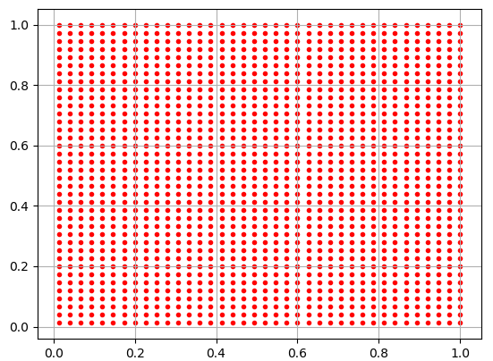
ar[2]
Out[2]: array([ 0.07 , 0.10246951, 0.04949747, 0.09899495], dtype=float32)
ar[3]
Out[3]: array([ 0.07 , 0.10246951, 0.09899495, 0.04949747], dtype=float32)
可以看到所有的中心点都分布在[0,1]区间,而ar[2]、ar[3]是搜索框宽高。
回过头来看函数体可以清楚看出来,
- 中心点和宽高都是放缩了的,乘300后才是对应于原图像的位置和宽高,这样层层下来,达到不同尺度不同位置的检测
-
中心点公式:y = (y.astype(dtype) + offset) * step / img_shape[0],实际上step*feat_shape约等于img_shape,
这使得网格点坐标介于0~1,放缩一下即可到图像大小,这也就是超参数anchor_steps的意义:用于辅助放缩搜
索网格中心点的位置 - 除了前两组宽高的计算不依赖anchor_ratios,后面的宽高计算中:
- h需要乘anchor_ratios**0.5
- w需要除anchor_ratios**0.5
且,感受野控制依赖两个参数:
anchor_sizes=[(21., 45.),
              (45., 99.),
              (99., 153.),
              (153., 207.),
              (207., 261.),
              (261., 315.)]
anchor_ratios=[[2, .5],
               [2, .5, 3, 1./3],
               [2, .5, 3, 1./3],
               [2, .5, 3, 1./3],
               [2, .5],
               [2, .5]]
至此,搜索网格生成完成,下一节,我们将从目标识别任务的数据处理入手,进一步了解SSD乃至其他目标检测网络的工作流程。