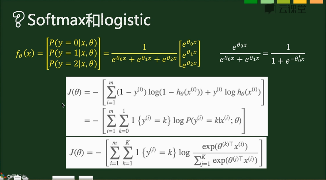
SoftMax实际上是Logistic的推广,当分类数为2的时候会退化为Logistic分类
其计算公式和损失函数如下,
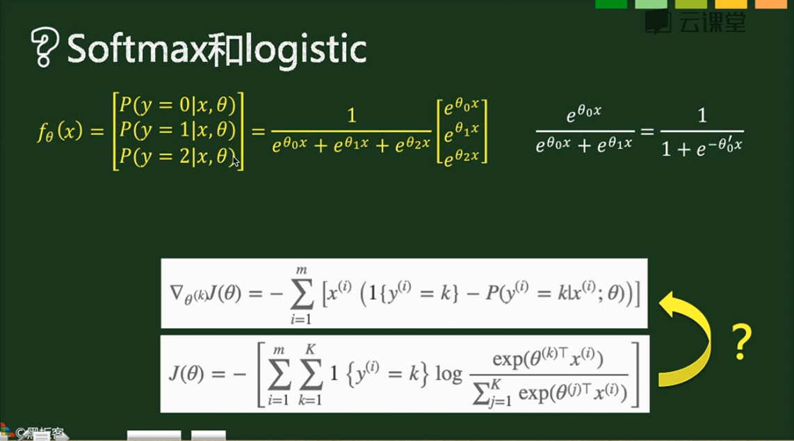
梯度如下,
1{条件} 表示True为1,False为0,在下图中亦即对于每个样本只有正确的分类才取1,对于损失函数实际上只有m个表达式(m个样本每个有一个正确的分类)相加,
对于梯度实际上是把我们以前的最后一层和分类层合并了:
- 第一步则和之前的求法类似,1-概率 & 0-概率组成向量,作为分类层的梯度,对batch数据实现的话就是建立一个(m,k)的01矩阵,直接点乘控制开关,最后求np.sum
- x的转置乘分类层梯度
- 全batch数据求和,实际上这在代码实现中和上一步放在了一块
对于单个数据梯度:x.T.dot(y_pred-y),维度是这样的(k,1)*(1,c)=(k,c)
对于成批数据梯度:X.T.dot(y_pred-y),维度是这样的(k,m)*(1,c)=(k,c),只不过结果矩阵的对应位置由x(i,1)*er(1,j)变换为x0(i,1)*er(1,j)+x1(i,1)*er(1,j)... ...正好是对全batch求了个和,所以后面需要除下去
X.T.dot(grad_next)结果是batch梯度累加和,所以需要除以样本数m,这个结论对全部使用本公式的梯度均成立(1,这句话是废话;2,但是几乎全部机器or深度学习算法都需要矩阵乘法,亦即梯度必须使用本公式,所以是很重要的废话)。
L2正则化:lamda*np.sum(W*W)或者lamda*np.sum(W.T.dot(W))均可,实际上就是W各个项的平方和
#计算Error,Cost,Grad
y_dash = self.softmax(X.dot(theta_n))   # 向前传播结果

Y = np.zeros((m,10))                    # one-hot编码label矩阵
for i in range(m):
    Y[i,y[i]]=1

error = np.sum(Y * np.log(y_dash), axis=1)   # 注意,这里是点乘
cost = -np.sum(error, axis=0)
grad = X.T.dot(y_dash-Y)

grad_n = grad.ravel()
代码实现:
import numpy as np
import matplotlib.pyplot as plt
import math

def scale_n(x):
    return x
    #return (x-x.mean(axis=0))/(x.std(axis=0)+1e-10)


class SoftMaxModel(object):
    def __init__(self,alpha=0.06,threhold=0.0005):
        self.alpha = alpha         # 学习率
        self.threhold = threhold   # 循环终止阈值
        self.num_classes = 10      # 分类数

    def setup(self,X):
        # 初始化权重矩阵,注意,由于是多分类,所以权重由向量变化为矩阵
        # 而且这里面初始化的是flat为1维的矩阵
        m, n = X.shape  # 400,15
        s = math.sqrt(6) / math.sqrt(n+self.num_classes)
        theta = np.random.rand(n*(self.num_classes))*2*s-s  #[15,1]
        return theta

    def softmax(self,x):
        # 先前传播softmax多分类
        # 注意输入的x是[batch数目n,类数目m],输出是[batch数目n,类数目m]
        e = np.exp(x)
        temp = np.sum(e, axis=1,keepdims=True)
        return e/temp

    def get_cost_grad(self,theta,X,y):
        m, n = X.shape
        theta_n = theta.reshape(n, self.num_classes)

        #计算Error,Cost,Grad
        y_dash = self.softmax(X.dot(theta_n))   # 向前传播结果

        Y = np.zeros((m,10))                    # one-hot编码label矩阵
        for i in range(m):
            Y[i,y[i]]=1

        error = np.sum(Y * np.log(y_dash), axis=1)
        cost = -np.sum(error, axis=0)
        grad = X.T.dot(y_dash-Y)

        grad_n = grad.ravel()
        return cost,grad_n


    def train(self,X,y,max_iter=50, batch_size=200):
        m, n = X.shape  # 400,15
        theta = self.setup(X)

        #our intial prediction
        prev_cost = None
        loop_num = 0
        n_samples = y.shape[0]
        n_batches = n_samples // batch_size
        # Stochastic gradient descent with mini-batches
        while loop_num < max_iter:
            for b in range(n_batches):
                batch_begin = b*batch_size
                batch_end = batch_begin+batch_size
                X_batch = X[batch_begin:batch_end]
                Y_batch = y[batch_begin:batch_end]


                #intial cost
                cost,grad = self.get_cost_grad(theta,X_batch,Y_batch)

                theta = theta- self.alpha * grad/float(batch_size)

            loop_num+=1
            if loop_num%10==0:
                print (cost,loop_num)
            if prev_cost:
                if prev_cost - cost <= self.threhold:
                    break

            prev_cost = cost


        self.theta = theta
        print (theta,loop_num)

    def train_scipy(self,X,y):
        m,n = X.shape
        import scipy.optimize
        options = {'maxiter': 50, 'disp': True}
        J = lambda x: self.get_cost_grad(x, X, y)
        theta = self.setup(X)

        result = scipy.optimize.minimize(J, theta, method='L-BFGS-B', jac=True, options=options)
        self.theta = result.x

    def predict(self,X):
        m,n = X.shape
        theta_n = self.theta.reshape(n, self.num_classes)
        a = np.argmax(self.softmax(X.dot(theta_n)),axis=1)
        return a


    def grad_check(self,X,y):
        epsilon = 10**-4
        m, n = X.shape

        sum_error=0
        N=300

        for i in range(N):
            theta = self.setup(X)
            j = np.random.randint(1,len(theta))
            theta1=theta.copy()
            theta2=theta.copy()
            theta1[j]+=epsilon
            theta2[j]-=epsilon

            cost1,grad1 = self.get_cost_grad(theta1,X,y)
            cost2,grad2 = self.get_cost_grad(theta2,X,y)
            cost3,grad3 = self.get_cost_grad(theta,X,y)

            sum_error += np.abs(grad3[j]-(cost1-cost2)/float(2*epsilon))
        print ("grad check error is %e
"%(sum_error/float(N)))


if __name__=="__main__":


    import cPickle, gzip
    # Load the dataset
    f = gzip.open('mnist.pkl.gz', 'rb')
    train_set, valid_set, test_set = cPickle.load(f)
    f.close()
    train_X = scale_n(train_set[0])
    train_y = train_set[1]
    test_X = scale_n(test_set[0])
    test_y = test_set[1]


    l_model = SoftMaxModel()

    l_model.grad_check(test_X[0:200,:],test_y[0:200])

    l_model.train_scipy(train_X,train_y)


    predict_train_y = l_model.predict(train_X)
    b = predict_train_y!=train_y

    error_train = np.sum(b, axis=0)/float(b.size)

    predict_test_y = l_model.predict(test_X)
    b = predict_test_y!=test_y

    error_test = np.sum(b, axis=0)/float(b.size)

    print ("Train Error rate = %.4f,
Test Error rate = %.4f
"%(error_train,error_test))
这里面有scipy的优化器应用,因为不是重点(暂时没有学习这个库的日程),所以标注出来,需要用优化器优化函数的时候记得有这么回事再深入学习即可:
def train_scipy(self,X,y):
        m,n = X.shape
        import scipy.optimize
        options = {'maxiter': 50, 'disp': True}
        J = lambda x: self.get_cost_grad(x, X, y)
        theta = self.setup(X)

        result = scipy.optimize.minimize(J, theta, method='L-BFGS-B', jac=True, options=options)
        self.theta = result.x
主要是提供了一些比较复杂的优化算法,而且是一个优化自建目标函数的demo,以后可能有所应用。