PCL 概况
官网教程: http://www.pointclouds.org/documentation/tutorials/walkthrough.php#walkthrough
主要模块如下:
滤波(filters)

-
直通滤波 它的作用是过滤掉在指定维度方向上取值不在给定值域内的点。直通滤波器的实现原理如下:首先,指定一个维度以及该维度下的值域,其次,遍历点云中的每个点,判断该点在指定维度上的取值是否在值域内,删除取值不在值域内的点,最后,遍历结束,留下的点即构成滤波后的点云。直通滤波器简单高效,适用于消除背景等操作。
pcl::PassThrough<PointT> pass;
pass.setFilterFieldName("z");
pass.setFilterLimits(0.7,1.3);
pass.setInputCloud(preprocess_cloud);
pass.filter(*preprocess_cloud);
条件滤波 与直通滤波器类似,它的作用是过滤掉点云中不满足给定条件的点,其实现原理也与直通滤波器类似,只是判断方式改变了。相比于直通滤波器,条件滤波器更加灵活,功能也更丰富,其优势主要体现在条件的定义上。我们可以依据点云的不同特征定义多种条件,例如,定义条件为点在x,y和z维度下的取值同时满足某个值域,则可以在指定3D空间内对点云进行裁剪。
pcl::ConditionalRemoval<PointT> condition;
//计算点云中的点分别在x,y,z轴向上的最大与最小取值
pcl::getMinMax3D(*preprocess_cloud,minPT,maxPT);
//示例,定义“与”条件,定义如下:y轴向从最低点向上0.14米范围与x轴向从中间点分别向两边取0.12米范围
pcl::ConditionAnd<PointT>::Ptr and_cond(new pcl::ConditionAnd<PointT>());
and_cond->addComparison(pcl::FieldComparison<PointT>::ConstPtr(new pcl::FieldComparison<PointT>("y",pcl::ComparisonOps::GT,minPT[1])));
and_cond->addComparison(pcl::FieldComparison<PointT>::ConstPtr(new pcl::FieldComparison<PointT>("y",pcl::ComparisonOps::LT,minPT[1]+0.14)));
and_cond->addComparison(pcl::FieldComparison<PointT>::ConstPtr(new pcl::FieldComparison<PointT>("x",pcl::ComparisonOps::GT,(minPT[0]+maxPT[0])/2-0.12)));
and_cond->addComparison(pcl::FieldComparison<PointT>::ConstPtr(new pcl::FieldComparison<PointT>("x",pcl::ComparisonOps::LT,(minPT[0]+maxPT[0])/2+0.12)));
//为条件滤波器设置条件
condition.setCondition(and_cond);
condition.setInputCloud(preprocess_cloud);
condition.filter(*preprocess_cloud);
-
统计滤波 主要作用是去除稀疏离群噪点。在采集点云的过程中,由于测量噪声的影响,会引入部分离群噪点,它们在点云空间中分布稀疏。在估算点云局部特征(例如计算采样点处的法向量和曲率变化率)时,这些噪点可能导致错误的计算结果,从而使点云配准等后期处理失败。统计滤波器的主要思想是假设点云中所有的点与其最近的k个邻居点的平均距离满足高斯分布,那么,根据均值和方差可确定一个距离阈值,当某个点与其最近k个点的平均距离大于这个阈值时,判定该点为离群点并去除。统计滤波器的实现原理如下:首先,遍历点云,计算每个点与其最近的k个邻居点之间的平均距离;其次,计算所有平均距离的均值μ与标准差σ,则距离阈值dmax可表示为dmax=μ+α×σ,α是一个常数,可称为比例系数,它取决于邻居点的数目;最后,再次遍历点云,剔除与k个邻居点的平均距离大于dmax的点。
pcl::StatisticalOutlierRemoval<PointT> Static; Static.setMeanK(100);//邻居点数目k Static.setStddevMulThresh(1.5);//比例系数α Static.setInputCloud(preprocess_cloud); Static.filter(*preprocess_cloud); -
体素滤波 主要作用是对点云进行降采样,可以在保证点云原有几何结构基本不变的前提下减少点的数量,多用于密集型点云的预处理中,以加快后续配准、重建等操作的执行速度。体素栅格滤波器的主要思想是在点云所在三维空间创建一个体素栅格,对于栅格内的每一个体素,以体素内所有点的重心近似代替体素中的点,最终,所有体素中的重心点组成滤波后的点云。通过体素的大小可以控制降采样的程度,体素越大,则滤波后的点云越稀疏。体素栅格滤波器的执行速度较慢,但是它能最大限度地保留点云原始的几何信息。
pcl::VoxelGrid<PointT> voxel;
voxel.setLeafSize(0.01f, 0.01f, 0.01f);//体素格的大小
voxel.setInputCloud(preprocess_cloud);
voxel.filter(*preprocess_cloud);
特征(features)


法线 曲率
-
点法线 表面法线是几何体面的重要属性。而点云数据集在真实物体的表面表现为一组定点样本。对点云数据集的每个点的法线估计,可以看作是对表面法线的近似推断。确定表面一点法线的问题近似于估计表面的一个相切面法线的问题,因此转换过来以后就变成一个最小二乘法平面拟合估计问题,最小特征值对应的特征向量即为法向量。
如果是有序图像,可以使用积分图像进行法线估计。要确定待估计点的最近邻集合,不管是用k近邻还是半径约束的方法,都将是计算量巨大的。如果输入的点云是有序点云,利用这种有序性可以明显加快表面法线估计的速度,积分图像正是为了利用点云有序性提高法线估计的速度而引入的。( 具体原理)
* #include <pcl/io/io.h> #include <pcl/io/pcd_io.h> #include <pcl/features/integral_image_normal.h> //法线估计类头文件 #include <pcl/visualization/cloud_viewer.h> #include <pcl/point_types.h> #include <pcl/features/normal_3d.h> int main () { //打开点云代码 pcl::PointCloud<pcl::PointXYZ>::Ptr cloud (new pcl::PointCloud<pcl::PointXYZ>); pcl::io::loadPCDFile ("table_scene_lms400.pcd", *cloud); //创建法线估计估计向量 pcl::NormalEstimation<pcl::PointXYZ, pcl::Normal> ne; ne.setInputCloud (cloud); //创建一个空的KdTree对象,并把它传递给法线估计向量 //基于给出的输入数据集,KdTree将被建立 pcl::search::KdTree<pcl::PointXYZ>::Ptr tree (new pcl::search::KdTree<pcl::PointXYZ> ()); ne.setSearchMethod (tree); //存储输出数据 pcl::PointCloud<pcl::Normal>::Ptr cloud_normals (new pcl::PointCloud<pcl::Normal>); //使用半径在查询点周围3厘米范围内的所有临近元素 ne.setRadiusSearch (0.03); //计算特征值 ne.compute (*cloud_normals); // cloud_normals->points.size ()应该与input cloud_downsampled->points.size ()有相同的尺寸 //可视化 pcl::visualization::PCLVisualizer viewer("PCL Viewer"); viewer.setBackgroundColor (0.0, 0.0, 0.0); viewer.addPointCloudNormals<pcl::PointXYZ,pcl::Normal>(cloud, cloud_normals); //视点默认坐标是(0,0,0)可使用 setViewPoint(float vpx,float vpy,float vpz)来更换 while (!viewer.wasStopped ()) { viewer.spinOnce (); } return 0; } -
曲率 PCL提供的不是严格意义上的曲率,它是用局部数据形状的垂直方向的变化程度之比来近似的。
也就是主成分分析得到的特征值之间的比较得到的。(计算曲率,需要先求法线)
#include <pcl/io/io.h>
#include <pcl/io/obj_io.h>
#include <pcl/PolygonMesh.h>
#include<pcl/ros/conversions.h>
#include <pcl/point_cloud.h>
#include <pcl/io/vtk_lib_io.h>//loadPolygonFileOBJ所属头文件;

#include<pcl/features/normal_3d.h>
#include<pcl/features/principal_curvatures.h>

vector<PCURVATURE> getModelCurvatures(string modelPath)
{
	pcl::PointCloud<pcl::PointXYZ>::Ptr cloud(new pcl::PointCloud<pcl::PointXYZ>);
	pcl::PolygonMesh mesh;
	pcl::io::loadPolygonFileOBJ(modelPath, mesh);
	pcl::fromPCLPointCloud2(mesh.cloud, *cloud);

	//计算法线
	pcl::NormalEstimation<pcl::PointXYZ, pcl::Normal> ne;
	ne.setInputCloud(cloud);
	pcl::search::KdTree<pcl::PointXYZ>::Ptr tree(new pcl::search::KdTree<pcl::PointXYZ>		 ());
	ne.setSearchMethod(tree); //设置搜索方法
	pcl::PointCloud<pcl::Normal>::Ptr cloud_normals(new pcl::PointCloud<pcl::Normal>);
	//ne.setRadiusSearch(0.05); //设置半径邻域搜索
	ne.setKSearch(5);
	ne.compute(*cloud_normals); //计算法向量

	//计算曲率
	pcl::PrincipalCurvaturesEstimation<pcl::PointXYZ, pcl::Normal, 		               	     pcl::PrincipalCurvatures>pc;
	pcl::PointCloud<pcl::PrincipalCurvatures>::Ptr cloud_curvatures(new                       pcl::PointCloud<pcl::PrincipalCurvatures>);
	pc.setInputCloud(cloud);
	pc.setInputNormals(cloud_normals);
	pc.setSearchMethod(tree);
	//pc.setRadiusSearch(0.05);
	pc.setKSearch(5);
	pc.compute(*cloud_curvatures);

	//获取曲率集
	vector<PCURVATURE> tempCV;
	POINT3F tempPoint;
	float curvature = 0.0;
	PCURVATURE pv;
	tempPoint.x = tempPoint.y = tempPoint.z=0.0;
	for (int i = 0; i < cloud_curvatures->size();i++){
		//平均曲率
		//curvature = ((*cloud_curvatures)[i].pc1 + (*cloud_curvatures)[i].pc2) / 2;
		//高斯曲率
		curvature = (*cloud_curvatures)[i].pc1 * (*cloud_curvatures)[i].pc2;
		//pv.cPoint = tempPoint;
		pv.index = i;
		pv.curvature = curvature;
		tempCV.insert(tempCV.end(),pv);
	}
	return tempCV;
}
关键点(Keypoints)
关键点也称为兴趣点,它是2D图像或是3D点云或者曲面模型上,可以通过定义检测标准来获取的具有稳定性、区别性的点集,从技术上来说,关键点的数量相比于原始点云或图像的数据量减小很多、关键点与局部特征描述子结合在一起组成关键点描述子,它常用来表示原始数据,而且不失代表性和描述性,从而加快了后续的识别、追踪等的速度。

- 边缘提取 点云的边缘又分为三种:前景边缘,背景边缘,阴影边缘。边缘提取原理
-
NARF(Normal Aligned Radial Feature) 关键点关键点提取
-
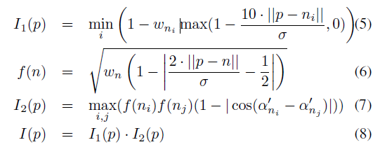
对于点云构成的曲面而言,某处的曲率无疑是一个非常重要的结构描述因素。某点的曲率越大,则该点处曲面变化越剧烈。在2D rangeImage 上,去 pi 点及其周边与之距离小于2deta的点,进行PCA主成分分析。可以得到一个 主方向v,以及曲率值 lamda. 注意, v 必然是一个三维向量。
-
那么对于边缘点,可以取其 权重 w 为1 , v 为边缘方向。
-
对于其他点,取权重 w 为 1-(1-lamda)^3 , 方向为 v 在平面 p上的投影。 平面 p 垂直于 pi 与原点连线。到此为止,每个点都有了两个量,一个权重,一个方向。将权重与方向带入下列式子 I 就是某点 为特征点的可能性。
-
NARF探测步骤如下:
- 遍历每个深度图像点,通过寻找在近邻区域有深度变化的位置进行边缘检测
- 遍历每个深度图像点,根据近邻区域的表面变化决定一测度表面变化的系数,及变化的主方向
- 根据第二步找到的主方向计算兴趣点特征,表征该方向和其他方向的不同,以及该处表面的变化情况(稳定性)
- 对兴趣值进行平滑滤波
- 进行无最大值压缩找到的最终关键点,即为NARF关键点
- 举例代码
-
include <iostream>

#include <boost/thread/thread.hpp>
#include <pcl/range_image/range_image.h>
#include <pcl/io/pcd_io.h>
#include <pcl/visualization/range_image_visualizer.h>
#include <pcl/visualization/pcl_visualizer.h>
#include <pcl/features/range_image_border_extractor.h>
#include <pcl/keypoints/narf_keypoint.h>
#include <pcl/features/narf_descriptor.h>
#include <pcl/console/parse.h>

typedef pcl::PointXYZ PointType;

// --------------------
// -----Parameters-----
// --------------------
float angular_resolution = 0.5f;           ////angular_resolution为模拟的深度传感器的角度分辨率,即深度图像中一个像素对应的角度大小
float support_size = 0.2f;                 //点云大小的设置
pcl::RangeImage::CoordinateFrame coordinate_frame = pcl::RangeImage::CAMERA_FRAME;     //设置坐标系
bool setUnseenToMaxRange = false;
bool rotation_invariant = true;

// --------------
// -----Help-----
// --------------
void
printUsage (const char* progName)
{
  std::cout << "

Usage: "<<progName<<" [options] <scene.pcd>

"
            << "Options:
"
            << "-------------------------------------------
"
            << "-r <float>   angular resolution in degrees (default "<<angular_resolution<<")
"
            << "-c <int>     coordinate frame (default "<< (int)coordinate_frame<<")
"
            << "-m           Treat all unseen points to max range
"
            << "-s <float>   support size for the interest points (diameter of the used sphere - "
                                                                  "default "<<support_size<<")
"
            << "-o <0/1>     switch rotational invariant version of the feature on/off"
            <<               " (default "<< (int)rotation_invariant<<")
"
            << "-h           this help
"
            << "

";
}

void
setViewerPose (pcl::visualization::PCLVisualizer& viewer, const Eigen::Affine3f& viewer_pose)  //设置视口的位姿
{
  Eigen::Vector3f pos_vector = viewer_pose * Eigen::Vector3f (0, 0, 0);   //视口的原点pos_vector
  Eigen::Vector3f look_at_vector = viewer_pose.rotation () * Eigen::Vector3f (0, 0, 1) + pos_vector;  //旋转+平移look_at_vector
  Eigen::Vector3f up_vector = viewer_pose.rotation () * Eigen::Vector3f (0, -1, 0);   //up_vector
  viewer.setCameraPosition (pos_vector[0], pos_vector[1], pos_vector[2],      //设置照相机的位姿
                            look_at_vector[0], look_at_vector[1], look_at_vector[2],
                            up_vector[0], up_vector[1], up_vector[2]);
}

// --------------
// -----Main-----
// --------------
int
main (int argc, char** argv)
{
  // --------------------------------------
  // -----Parse Command Line Arguments-----
  // --------------------------------------
  if (pcl::console::find_argument (argc, argv, "-h") >= 0)
  {
    printUsage (argv[0]);
    return 0;
  }
  if (pcl::console::find_argument (argc, argv, "-m") >= 0)
  {
    setUnseenToMaxRange = true;
    cout << "Setting unseen values in range image to maximum range readings.
";
  }
  if (pcl::console::parse (argc, argv, "-o", rotation_invariant) >= 0)
    cout << "Switching rotation invariant feature version "<< (rotation_invariant ? "on" : "off")<<".
";
  int tmp_coordinate_frame;
  if (pcl::console::parse (argc, argv, "-c", tmp_coordinate_frame) >= 0)
  {
    coordinate_frame = pcl::RangeImage::CoordinateFrame (tmp_coordinate_frame);
    cout << "Using coordinate frame "<< (int)coordinate_frame<<".
";
  }
  if (pcl::console::parse (argc, argv, "-s", support_size) >= 0)
    cout << "Setting support size to "<<support_size<<".
";
  if (pcl::console::parse (argc, argv, "-r", angular_resolution) >= 0)
    cout << "Setting angular resolution to "<<angular_resolution<<"deg.
";
  angular_resolution = pcl::deg2rad (angular_resolution);

  // ------------------------------------------------------------------
  // -----Read pcd file or create example point cloud if not given-----
  // ------------------------------------------------------------------
  pcl::PointCloud<PointType>::Ptr point_cloud_ptr (new pcl::PointCloud<PointType>);
  pcl::PointCloud<PointType>& point_cloud = *point_cloud_ptr;
  pcl::PointCloud<pcl::PointWithViewpoint> far_ranges;
  Eigen::Affine3f scene_sensor_pose (Eigen::Affine3f::Identity ());
  std::vector<int> pcd_filename_indices = pcl::console::parse_file_extension_argument (argc, argv, "pcd");
  if (!pcd_filename_indices.empty ())
  {
    std::string filename = argv[pcd_filename_indices[0]];
    if (pcl::io::loadPCDFile (filename, point_cloud) == -1)
    {
      cerr << "Was not able to open file ""<<filename<<"".
";
      printUsage (argv[0]);
      return 0;
    }
    scene_sensor_pose = Eigen::Affine3f (Eigen::Translation3f (point_cloud.sensor_origin_[0], //场景传感器的位置
                                                               point_cloud.sensor_origin_[1],
                                                               point_cloud.sensor_origin_[2])) *
                        Eigen::Affine3f (point_cloud.sensor_orientation_);
    std::string far_ranges_filename = pcl::getFilenameWithoutExtension (filename)+"_far_ranges.pcd";
    if (pcl::io::loadPCDFile (far_ranges_filename.c_str (), far_ranges) == -1)
      std::cout << "Far ranges file ""<<far_ranges_filename<<"" does not exists.
";
  }
  else
  {
    setUnseenToMaxRange = true;
    cout << "
No *.pcd file given => Genarating example point cloud.

";
    for (float x=-0.5f; x<=0.5f; x+=0.01f)
    {
      for (float y=-0.5f; y<=0.5f; y+=0.01f)
      {
        PointType point;  point.x = x;  point.y = y;  point.z = 2.0f - y;
        point_cloud.points.push_back (point);
      }
    }
    point_cloud.width = (int) point_cloud.points.size ();  point_cloud.height = 1;
  }

  // -----------------------------------------------
  // -----Create RangeImage from the PointCloud-----
  // -----------------------------------------------
  float noise_level = 0.0;
  float min_range = 0.0f;
  int border_size = 1;
  boost::shared_ptr<pcl::RangeImage> range_image_ptr (new pcl::RangeImage);
  pcl::RangeImage& range_image = *range_image_ptr;
  range_image.createFromPointCloud (point_cloud, angular_resolution, pcl::deg2rad (360.0f), pcl::deg2rad (180.0f),
                                   scene_sensor_pose, coordinate_frame, noise_level, min_range, border_size);
  range_image.integrateFarRanges (far_ranges);
  if (setUnseenToMaxRange)
    range_image.setUnseenToMaxRange ();

  // --------------------------------------------
  // -----Open 3D viewer and add point cloud-----
  // --------------------------------------------
  pcl::visualization::PCLVisualizer viewer ("3D Viewer");
  viewer.setBackgroundColor (1, 1, 1);
  pcl::visualization::PointCloudColorHandlerCustom<pcl::PointWithRange> range_image_color_handler (range_image_ptr, 0, 0, 0);
  viewer.addPointCloud (range_image_ptr, range_image_color_handler, "range image");
  viewer.setPointCloudRenderingProperties (pcl::visualization::PCL_VISUALIZER_POINT_SIZE, 1, "range image");
  //viewer.addCoordinateSystem (1.0f, "global");
  //PointCloudColorHandlerCustom<PointType> point_cloud_color_handler (point_cloud_ptr, 150, 150, 150);
  //viewer.addPointCloud (point_cloud_ptr, point_cloud_color_handler, "original point cloud");
  viewer.initCameraParameters ();
  setViewerPose (viewer, range_image.getTransformationToWorldSystem ());

  // --------------------------
  // -----Show range image-----
  // --------------------------
  pcl::visualization::RangeImageVisualizer range_image_widget ("Range image");
  range_image_widget.showRangeImage (range_image);
  /*********************************************************************************************************
   创建RangeImageBorderExtractor对象,它是用来进行边缘提取的,因为NARF的第一步就是需要探测出深度图像的边缘,   *********************************************************************************************************/
  // --------------------------------
  // -----Extract NARF keypoints-----
  // --------------------------------
  pcl::RangeImageBorderExtractor range_image_border_extractor;   //用来提取边缘
  pcl::NarfKeypoint narf_keypoint_detector;      //用来检测关键点
  narf_keypoint_detector.setRangeImageBorderExtractor (&range_image_border_extractor);   //
  narf_keypoint_detector.setRangeImage (&range_image);
  narf_keypoint_detector.getParameters ().support_size = support_size;    //设置NARF的参数

  pcl::PointCloud<int> keypoint_indices;
  narf_keypoint_detector.compute (keypoint_indices);
  std::cout << "Found "<<keypoint_indices.points.size ()<<" key points.
";

  // ----------------------------------------------
  // -----Show keypoints in range image widget-----
  // ----------------------------------------------
  //for (size_t i=0; i<keypoint_indices.points.size (); ++i)
    //range_image_widget.markPoint (keypoint_indices.points[i]%range_image.width,
                                  //keypoint_indices.points[i]/range_image.width);

  // -------------------------------------
  // -----Show keypoints in 3D viewer-----
  // -------------------------------------
  pcl::PointCloud<pcl::PointXYZ>::Ptr keypoints_ptr (new pcl::PointCloud<pcl::PointXYZ>);

  pcl::PointCloud<pcl::PointXYZ>& keypoints = *keypoints_ptr;

  keypoints.points.resize (keypoint_indices.points.size ());
  for (size_t i=0; i<keypoint_indices.points.size (); ++i)

    keypoints.points[i].getVector3fMap () = range_image.points[keypoint_indices.points[i]].getVector3fMap ();

  pcl::visualization::PointCloudColorHandlerCustom<pcl::PointXYZ> keypoints_color_handler (keypoints_ptr, 0, 255, 0);
  viewer.addPointCloud<pcl::PointXYZ> (keypoints_ptr, keypoints_color_handler, "keypoints");
  viewer.setPointCloudRenderingProperties (pcl::visualization::PCL_VISUALIZER_POINT_SIZE, 7, "keypoints");

  // ------------------------------------------------------
  // -----Extract NARF descriptors for interest points-----
  // ------------------------------------------------------
  std::vector<int> keypoint_indices2;
  keypoint_indices2.resize (keypoint_indices.points.size ());
  for (unsigned int i=0; i<keypoint_indices.size (); ++i) // This step is necessary to get the right vector type
    keypoint_indices2[i]=keypoint_indices.points[i];
  pcl::NarfDescriptor narf_descriptor (&range_image, &keypoint_indices2);
  narf_descriptor.getParameters ().support_size = support_size;
  narf_descriptor.getParameters ().rotation_invariant = rotation_invariant;
  pcl::PointCloud<pcl::Narf36> narf_descriptors;
  narf_descriptor.compute (narf_descriptors);
  cout << "Extracted "<<narf_descriptors.size ()<<" descriptors for "
                      <<keypoint_indices.points.size ()<< " keypoints.
";

  //--------------------
  // -----Main loop-----
  //--------------------
  while (!viewer.wasStopped ())
  {
    range_image_widget.spinOnce ();  // process GUI events
    viewer.spinOnce ();
    pcl_sleep(0.01);
  }
}
配准(Registration)
给定两个来自不同坐标系的三维数据点集,找到两个点集空间的变换关系,使得两个点集能统一到同一坐标系统中,即配准过程。配准的目标是在全局坐标框架中找到单独获取的视图的相对位置和方向,使得它们之间的相交区域完全重叠。


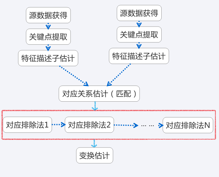
方法一: 两两配准(pairwise registration )
对点云数据集的配准问题是两两配准(pairwise registration 或 pair-wise registration)。通常通过一个估计得到的平移矩阵和的4*4的变换矩阵使得一个点云的数据集精确的与另一个点云数据集(目标数据集)进行完美的配准。具体的实现步骤是:
- 首先从两个数据集中按照同样的关键点选取的标准,提取关键点
- 对选择所有的关键点分别计算其特征描述子
- 结合特征描述子在两个数据集中的坐标位置,以两者之间的特征和位置的相似度为基础,来估算它们的对应关系,初步得到估计对应点对
- 假设数据是有噪声,除去对配准有影响的错误的对应点对
- 利用剩余的正确的对应关系来估算刚体变换,完整配准
- 特征点配准实例
方法二:迭代最近点 Iterative Closest Point (ICP)
ICP算法本质上是基于最小二乘法的最优配准方法。该算法重复进行选择对应关系点对,计算最优刚体变换这一过程,直到满足正确配准的收敛精度要求。ICP是一个广泛使用的配准算法,主要目的就是找到旋转和平移参数,将两个不同坐标系下的点云,以其中一个点云坐标系为全局坐标系,另一个点云经过旋转和平移后两组点云重合部分完全重叠。ICP算法最早由Chen and Medioni,and Besl and McKay提出。
算法的输入:参考点云和目标点云,停止迭代的标准。
算法的输出:旋转和平移矩阵,即转换矩阵。
基本过程:
- 对于目标点云中的每个点,匹配参考点云(或选定集合)中的最近点。
- 求得使上述对应点对计算均方根(root mean square,RMS)最小的刚体变换,求得平移参数和旋转参数
- 使用获得的转换矩阵来转换目标点云。
- 迭代(重新关联点),直到满足终止迭代的条件(迭代次数或误差小于阈值)。这里的误差最小,可以是相邻两次均方根差的绝对值小于某一限差。
举例:
void PairwiseICP(const pcl::PointCloud<PointT>::Ptr &cloud_target, const pcl::PointCloud<PointT>::Ptr &cloud_source, pcl::PointCloud<PointT>::Ptr &output )
{
	PointCloud<PointT>::Ptr src(new PointCloud<PointT>);
	PointCloud<PointT>::Ptr tgt(new PointCloud<PointT>);

	tgt = cloud_target;
	src = cloud_source;

	pcl::IterativeClosestPoint<PointT, PointT> icp;
	icp.setMaxCorrespondenceDistance(0.1);
	icp.setTransformationEpsilon(1e-10);
	icp.setEuclideanFitnessEpsilon(0.01);
	icp.setMaximumIterations (100);

	icp.setInputSource (src);
	icp.setInputTarget (tgt);
	icp.align (*output);

//	std::cout << "has converged:" << icp.hasConverged() << " score: " <<icp.getFitnessScore() << std::endl;


	output->resize(tgt->size()+output->size());
	for (int i=0;i<tgt->size();i++)
	{
		output->push_back(tgt->points[i]);
	}
	cout<<"After registration using ICP:"<<output->size()<<endl;

}
//setMaximumIterations, 最大迭代次数,icp是一个迭代的方法,最多迭代这些次;
//setTransformationEpsilon, 前一个变换矩阵和当前变换矩阵的差异小于阈值时,就认为已经收敛了,是一条收敛条件;
//setEuclideanFitnessEpsilon, 还有一条收敛条件是均方误差和小于阈值, 停止迭代
KD树(KD-TREE)

插入
先以一个简单直观的实例来介绍k-d树算法。假设有6个二维数据点{(2,3),(5,4),(9,6),(4,7),(8,1),(7,2)},数据点 位于二维空间内(如图1中黑点所示)。k-d树算法就是要确定图1中这些分割空间的分割线(多维空间即为分割平面,一般为超平面)。下面就要通过一步步展 示k-d树是如何确定这些分割线的。

由于此例简单,数据维度只有2维,所以可以简单地给x,y两个方向轴编号为0,1,也即split={0,1}。
(1)确定split域的首先该取的值。分别计算x,y方向上数据的方差得知x方向上的方差最大,所以split域值首先取0,也就是x轴方向;
(2)确定Node-data的域值。根据x轴方向的值2,5,9,4,8,7排序选出中值为7,所以Node-data = (7,2)。这样,该节点的分割超平面就是通过(7,2)并垂直于split = 0(x轴)的直线x = 7;
(3)确定左子空间和右子空间。分割超平面x = 7将整个空间分为两部分,如图2所示。x < = 7的部分为左子空间,包含3个节点{(2,3),(5,4),(4,7)};另一部分为右子空间,包含2个节点{(9,6),(8,1)}。
(4)k-d树的构建是一个递归的过程。然后对左子空间和右子空间内的数据重复根节点的过程就可以得到下一级子节点(5,4)和(9,6)(也就是 左右子空间的'根'节点),同时将空间和数据集进一步细分。如此反复直到空间中只包含一个数据点,如图1所示。最后生成的k-d树如图3所示。
搜索
给定点p,查询数据集中与其距离最近点的过程即为最近邻搜索。
如在上文构建好的k-d tree上搜索(3,5)的最近邻时,本文结合如下左右两图对二维空间的最近邻搜索过程作分析。
a)首先从根节点(7,2)出发,将当前最近邻设为(7,2),对该k-d tree作深度优先遍历。以(3,5)为圆心,其到(7,2)的距离为半径画圆(多维空间为超球面),可以看出(8,1)右侧的区域与该圆不相交,所以(8,1)的右子树全部忽略。
b)接着走到(7,2)左子树根节点(5,4),与原最近邻对比距离后,更新当前最近邻为(5,4)。以(3,5)为圆心,其到(5,4)的距离为半径画圆,发现(7,2)右侧的区域与该圆不相交,忽略该侧所有节点,这样(7,2)的整个右子树被标记为已忽略。
c)遍历完(5,4)的左右叶子节点,发现与当前最优距离相等,不更新最近邻。所以(3,5)的最近邻为(5,4)。

八叉树(Octree)
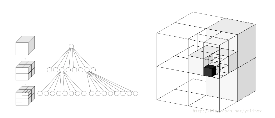
八叉树库提供了从点云数据创建层次树数据结构的有效方法。这样就可以对点数据集执行空间分区、下采样和搜索操作。每个八叉树节点要么有八个子节点要么没有子节点。根节点描述了一个封装所有点的立方体边界框。在每个树级别,该空间被2的因子细分,从而提高体素分辨率。
八叉树实现提供了高效的近邻搜索例程,如“体素内近邻搜索”、“K近邻搜索”和“半径内近邻搜索”。它会根据点数据集自动调整其尺寸。一组叶节点类提供了额外的功能,例如空间“占用率”和“每个体素的点密度”检查。用于序列化和反序列化的函数能够有效地将八叉树结构编码为二进制格式。此外,在需要高速创建八叉树的情况下,内存池实现减少了昂贵的内存分配和释放操作。
下图显示了最低树级别八叉树节点的体素边界框。八叉树体素围绕着斯坦福兔子表面的每一个三维点。红点代表点数据。此图像是用八叉树查看器创建的。

想象我们有一个房间,房间里某个角落藏着一枚金币,我们想很快的把金币找出来,聪明的你会怎 么做?我们可以把房间当成一个立方体,先切成八个小立方体,然后排除掉没有放任何东西的小立方体,再把有可能藏金币的小立方体继续切八等份….如此下去, 平均在Log8(房间内的所有物品数)的时间内就可找到金币。因此,八叉树就是用在3D空间中的场景管理,可以很快地知道物体在3D场景中的位置,或侦测 与其它物体是否有碰撞以及是否在可视范围内。
实现八叉树的原理
(1). 设定最大递归深度。
(2). 找出场景的最大尺寸,并以此尺寸建立第一个立方体。
(3). 依序将单位元元素丢入能被包含且没有子节点的立方体。
(4). 若没达到最大递归深度,就进行细分八等份,再将该立方体所装的单位元元素全部分担给八个子立方体。
(5). 若发现子立方体所分配到的单位元元素数量不为零且跟父立方体是一样的,则该子立方体停止细分,因为跟据空间分割理论,细分的空间所得到的分配必定较少,若是一样数目,则再怎么切数目还是一样,会造成无穷切割的情形。
(6). 重复3,直到达到最大递归深度。
分割(Segmentation)
分割库包含将点云分割为不同簇的算法。这些算法最适合处理由许多空间隔离区域组成的点云。在这种情况下,聚类通常用于将云分解为其组成部分,然后可以独立处理。
解释聚类方法如何工作的理论入门可以在集群抽取教程中找到。这两幅图展示了平面模型分割(左)和圆柱模型分割(右)的结果。

样本一致性(Sample Consensus)
sample_consensus库保存sample consensus(SAC)方法,如RANSAC和模型,如平面和圆柱体。它们可以自由组合以检测点云中的特定模型及其参数。
解释样本一致性算法如何工作的理论入门可以在随机样本一致性教程中找到
此库中实现的一些模型包括:直线、平面、圆柱体和球体。平面拟合通常用于检测常见的室内表面,如墙壁、地板和桌面。其他模型可用于检测和分割具有常见几何结构的对象(例如,将圆柱体模型拟合到杯子上)。

表面(Surface)
曲面库处理从三维扫描重建原始曲面。根据手头的任务,这可以是外壳线、网格表示或具有法线的平滑/重采样曲面。
如果云是有噪声的,或者云是由多个未完全对齐的扫描组成,平滑和重采样可能很重要。根据需要,可以调整曲面估计的复杂度,并在同一步骤中估计出法线。

范围图像(Range Image)
range_图像库包含两个类,用于表示和处理range图像。范围图像(或深度贴图)是其像素值表示距离传感器原点的距离或深度的图像。距离图像是一种常见的三维表示,通常由立体或飞行时间摄像机生成。通过了解摄像机的内在校准参数,可以将距离图像转换为点云。
注意:range_图像现在是公共模块的一部分。

可视化(Visualization)
可视化库的建立是为了能够快速原型化和可视化算法在三维点云数据上的运行结果。与OpenCV在屏幕上显示2D图像和绘制基本2D形状的highgui例程类似。
