%%%%%%%%%%%%%%%%%%%%%%%%%%%%%%%%%
clear all;clc;
%%%%%%%%%%%%%%%%%%%%%%%%%%%%%%%%%%%%%%%%%%%%%%%%%%%%%%%%%%%%%%%%%%
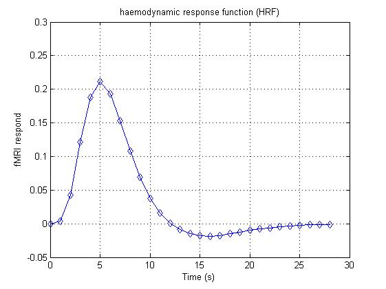
% haemodynamic response function: BOLD signal has stereotyped shape every
% time a stimulus hits it. We usually use the spm_hrf.m in SPM toolbox to
% produce HRF. Here, we use the 29 vector to represent HRF from 0 s to
% 28 s. In this simulation, we suppose TR=1 s.
HRF = [0 0.004 0.043 0.121 0.188 0.211 0.193 0.153 0.108 0.069 0.038 0.016 0.001 -0.009 -0.015 -0.018 -0.019 -0.018 -0.015 -0.013 -0.010 -0.008 -0.006 -0.004 -0.003 -0.002 -0.001 -0.001 -0.001];
% We will plot its shape with figure 1:
figure(1)
% here is the x-coordinates
t = [0:28];
plot(t,HRF,'d-');
grid on;
xlabel('Time (s)');
ylabel('fMRI respond');
title('haemodynamic response function (HRF)');
结果:
%%%%%%%%%%%%%%%%%%%%%%%%%%%%%%%%%%%%%%%%%%%%%%%%%%%%%%%%%%%%%%%%%%
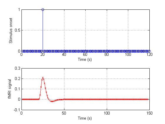
% Suppose that our scan for 120 s, we will have 120 point (because TR = 1
% s). If a stimulus onset at t=20 s, we can use a vector to represent this
% stimulation.
onset_1 = [zeros(1,19) 1 zeros(1,100)];
% i.e. the whole vector is maked with 19 zeros, a single 1, and then 100
% zeros. As we have the stimulus onset vector and HRF we can convolve them.
% In Matlab, the command to convolve two vectors is "conv":
conv_1 = conv(HRF,onset_1);
% Let's plot the result in figure 2
figure(2);
% This figure will have 2 rows of subplots.
subplot(2,1,1);
% "Stem" is a good function for showing discrete events:
stem(onset_1);
grid on;
xlabel('Time (s)');
ylabel('Stimulus onset');
subplot(2,1,2);
plot(conv_1,'rx-');
grid on;
xlabel('Time (s)');
ylabel('fMRI signal');
结果:
%%%%%%%%%%%%%%%%%%%%%%%%%%%%%%%%%%%%%%%%%%%%%%%%%%%%%%%%%%%%%%%%%%
% Usually, we have repeat a task many times in a run. If three stimulus
% onsets at t=20, 50, 80 s, we also can use a vector to represent this
% stimulation.
onset_2 = [zeros(1,19) 1 zeros(1,29) 1 zeros(1,29) 1 zeros(1,20)];
% Here we use the conv again:
conv_2 = conv(HRF,onset_2);
% Let's plot the result in figure 3
figure(3);
% This figure will have 2 rows of subplots.
subplot(2,1,1);
% "Stem" is a good function for showing discrete events:
stem(onset_2);
grid on;
xlabel('Time (s)');
ylabel('Stimulus onset');
subplot(2,1,2);
plot(conv_2,'rx-');
grid on;
xlabel('Time (s)');
ylabel('fMRI signal');
结果: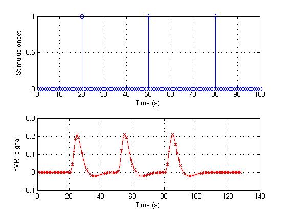
%%%%%%%%%%%%%%%%%%%%%%%%%%%%%%%%%%%%%%%%%%%%%%%%%%%%%%%%%%%%%%%%%%
% Now let's think about the fast event design. In this condition, we will
% have many task during a short time. If three stimulus onsets at t=20, 25,
% 30 s:
onset_3 = [zeros(1,19) 1 zeros(1,4) 1 zeros(1,4) 1 zeros(1,70)];
conv_3 = conv(HRF,onset_3);
figure(4);
subplot(2,1,1);
stem(onset_3);
grid on;
xlabel('Time (s)');
ylabel('Stimulus onset');
subplot(2,1,2);
plot(conv_3,'rx-');
grid on;
xlabel('Time (s)');
ylabel('fMRI signal');
结果:
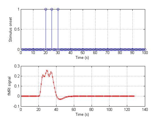
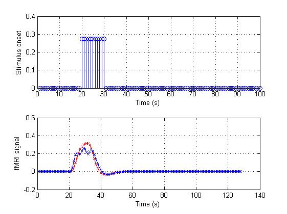
% The three events are so closed, the result signal is like a blocked
% design. Such as:
onset_4 = [zeros(1,19) ones(1,11) zeros(1,70)]*(3/11);
conv_4 = conv(HRF,onset_4);
figure(5);
subplot(2,1,1);
stem(onset_4);
grid on;
xlabel('Time (s)');
ylabel('Stimulus onset');
subplot(2,1,2);
plot(conv_4,'rx-');
% We will compare the result
hold on; % plot more than one time on a figure
plot(conv_3,'bx-');
grid on;
xlabel('Time (s)');
ylabel('fMRI signal');
结果: