朴素贝叶斯分类算法：具体内容

了解完了什么是贝叶斯公式后，我们开始接触这个算法的核心。

因为是要用Python实现的，所以我找到了skit-learn的官网，上面有朴素贝叶斯分类算法的帮助文档，看完之后感觉思路挺清晰的，这是网址： http://scikit-learn.org/stable/modules/naive_bayes.html

Naive Bayes methods are a set of supervised learning algorithms based on applying Bayes’ theorem with the “naive” assumption of independence between every pair of features. Given a class variable $y$ and a dependent feature vector $x_1$ through $x_n$ , Bayes’ theorem states the following relationship:

朴素贝叶斯方法是一组基于贝叶斯定理的有监督的学习算法，并且对各个特征之间有着“朴素”的假设：各个特征之间相互独立

对于给出的类别变量 $y$ 和相关的特征向量 $x_1$ 到 $x_n$ ，贝叶斯定理描述了以下关系：

$P(y mid x_1, dots, x_n) = frac{P(y) P(x_1, dots x_n mid y)} {P(x_1, dots, x_n)}$

Using the naive independence assumption that

使用朴素的独立假设，那么就有：

$P(x_i | y, x_1, dots, x_{i-1}, x_{i+1}, dots, x_n) = P(x_i | y),$

for all $i$ , this relationship is simplified to

对于所有的 $i$ ，贝叶斯定理就简化成了：

$P(y mid x_1, dots, x_n) = frac{P(y) prod_{i=1}^{n} P(x_i mid y)} {P(x_1, dots, x_n)}$

Since $P(x_1, dots, x_n)$ is constant given the input, we can use the following classification rule:

因为 $P(x_1, dots, x_n)$ 是常量（这个概率应该就是这一类在训练集中所占的比率，比如说训练集分两个类别，1类有1个特征向量，2类有两个，则P(1类)=1/3），我们可以用一下的分类规则：

$P(y mid x_1, dots, x_n) propto P(y) prod_{i=1}^{n} P(x_i mid y) Downarrow hat{y} = argmax_y P(y) prod_{i=1}^{n} P(x_i mid y),$

and we can use Maximum A Posteriori (MAP) estimation to estimate $P(y)$ and $P(x_i mid y)$ ; the former is then the relative frequency of class $y$ in the training set.

然后我们可以用最大后验估计（MAP）去估计 $P(y)$ 和 $P(x_i mid y)$ ；前者（即 $P(y)$ ）是 $y$ 类在训练集中的频率。

The different naive Bayes classifiers differ mainly by the assumptions they make regarding the distribution of $P(x_i mid y)$ .

不同的贝叶斯分类器主要区分在对 $P(x_i mid y)$ 的分布的假设上。

In spite of their apparently over-simplified assumptions, naive Bayes classifiers have worked quite well in many real-world situations, famously document classification and spam filtering. They require a small amount of training data to estimate the necessary parameters. (For theoretical reasons why naive Bayes works well, and on which types of data it does, see the references below.)

尽管朴素贝叶斯的假设（即各个特征之间相互独立）过于“朴素”，但是它仍然在现实应用中有着非常不错的效果，在文档分类和垃圾邮件过滤上非常出名。它只需要少部分的训练数据去估计必要的参数。（至于理论上的朴素贝叶斯那么出色的原因以及它应用在哪种类型上的数据，看一下以下参考）

Naive Bayes learners and classifiers can be extremely fast compared to more sophisticated methods. The decoupling of the class conditional feature distributions means that each distribution can be independently estimated as a one dimensional distribution. This in turn helps to alleviate problems stemming from the curse of dimensionality.

朴素贝叶斯学习者和分类器对比于其他的更为复杂精妙的方法，它的速度是非常之快的（可能是判断速度吧。。。）。下面这句真不会了。。好像是说有什么什么好处，能够避免维度灾难。

On the flip side, although naive Bayes is known as a decent classifier, it is known to be a bad estimator, so the probability outputs from predict_proba are not to be taken too seriously.

但是反过来说，尽管朴素贝叶斯是一个很好的分类器，它同时也是一个差劲的估计者（不会），所以来自predict_proba的概率输出是不严格的。

朴素贝叶斯分类器有三种模型，分别是高斯、多项式分布和伯努利。

因为我要用的是多项式，所以这里只介绍一下多项式分布模型：

MultinomialNB implements the naive Bayes algorithm for multinomially distributed data, and is one of the two classic naive Bayes variants used in text classification (where the data are typically represented as word vector counts, although tf-idf vectors are also known to work well in practice). The distribution is parametrized by vectors $heta_y = ( heta_{y1},ldots, heta_{yn})$ for each class $y$ , where $n$ is the number of features (in text classification, the size of the vocabulary) and $heta_{yi}$ is the probability $P(x_i mid y)$ of feature $i$ appearing in a sample belonging to class $y$ .

MultionomiaNB执行对多项式分布数据的贝叶斯算法，它是两个经典的用于文本分类（在文本分类中数据通常是由词频向量代表，尽管tf-idf向量同样在实战中效果显著）的朴素贝叶斯变形体之一。对于每个类别 $y$ ，它的分布已经被向量 $heta_y = ( heta_{y1},ldots, heta_{yn})$ 参数化了， $n$ 是特征的数量（在文本分类中则是词的大小...我估计应该是词频的意思）并且 $heta_{yi}$ 是特征 $i$ 在属于 $y$ 类的样本中出现的概率 $P(x_i mid y)$ 。

The parameters $heta_y$ is estimated by a smoothed version of maximum likelihood, i.e. relative frequency counting:

参数 $heta_y$ 已经由平滑的最大似然故意确定了，也就是说相关频率计数：

$hat{ heta}_{yi} = frac{ N_{yi} + alpha}{N_y + alpha n}$

where $N_{yi} = sum_{x in T} x_i$ is the number of times feature $i$ appears in a sample of class $y$ in the training set $T$ , and $N_{y} = sum_{i=1}^{|T|} N_{yi}$ is the total count of all features for class $y$ .

$N_{yi} = sum_{x in T} x_i$ 是特征 $i$ 在 $y$ 类的训练集样本中出现的次数， $N_{y} = sum_{i=1}^{|T|} N_{yi}$ 是 $y$ 类中所有的特征数

The smoothing priors $alpha ge 0$ accounts for features not present in the learning samples and prevents zero probabilities in further computations. Setting $alpha = 1$ is called Laplace smoothing, while $alpha < 1$ is called Lidstone smoothing.

平滑先验 $alpha ge 0$ 是为了解决一些没有出现在学习样本中的特征，防止在以后的计算中出现0概率。令 $alpha = 1$ 被称为拉普拉斯平滑处理，当 $alpha < 1$ 时被称为Lidstone平滑。

------------------------------------------------------------------------------------------------分割线----------------------------------------------------------------------------------------

所以在算法的实现方面，我们主要是去计算 $hat{ heta}_{yi} = frac{ N_{yi} + alpha}{N_y + alpha n}$ 这个参数，怎么样计算上面已经写明白了。但是有一些地方我还是不太明白，好在还有例子可以看看。

以下是例子的代码：

1 import numpy as np
2 x = np.random.randint(5,size=(6,100)) # 参数size代表6行100列，且1<=x<5
3 y=np.array([1,2,3,4,5,6])
4 from sklearn.naive_bayes import MultinomialNB
5 clf = MultinomialNB()
6 clf.fit(x, y)
7 print(clf.predict(x[2:3]))

结果：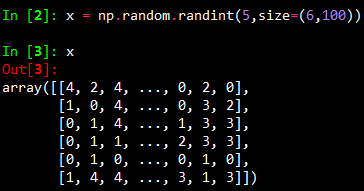

x应该就是训练集，y是类集合

自己再写个简单点的检验一下：

1 x2 = np.random.randint(6,size = (6,10))
2 y2 = np.array([1,2,3,4,5,6])
3 clf.fit(x2,y2)
4 print(clf.predict([0,3,4,1,4,7,5,4,5,4]))

结果：

看看第四类长什么样子：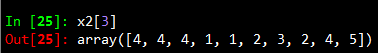

然而我是按照第一类去改写被预测的向量的

.......看来和我想的并不是一样的，看看能不能找得到帮助文档吧

http://scikit-learn.org/stable/modules/generated/sklearn.naive_bayes.MultinomialNB.html#sklearn.naive_bayes.MultinomialNB 这是MultinomialNB函数的帮助文档

仿佛看到了宝藏...好开心啊，赶紧点进去看看。看了许久，感觉自己的猜测应该是正确的

https://zhuanlan.zhihu.com/p/25984744 这个哥们写的值得参考，但是我觉得有点乱，就没怎么看了

决定自己再试试

1 x3 = np.random.randint(6,size = (6,8))
2 y3 = np.array([1,1,1,1,2,2])
3 clf.fit(x3,y3)
4 print(clf.predict([3,0,1,2,4,0,3,2]))

结果：

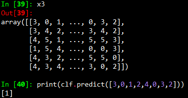
现在能够确定x就是训练集特征向量的一个数组，而y就是训练集的类集合的一个数组

所以使用朴素贝叶斯分类器主要的工作量都是在文本的预处理上，得到了特征向量后，只要选出训练样本，将训练样本转化为特征向量的一个数组就ok了。

如果上面有哪些地方不对的，还请各位看官老爷指出来~~~