[读书笔记]机器学习：实用案例解析（1）

第1章使用R语言

#machine learing for heckers
#chapter 1

library(ggplot2)
library(plyr)

#.tsv文件用制表符进行分割
#字符串默认为factor类型，因此stringsAsFactors置FALSE防止转换
#header置FALSE防止将第一行当做表头
#定义空字符串为NA：na.strings = ""

ufo <- read.delim("ML_for_Hackers/01-Introduction/data/ufo/ufo_awesome.tsv", 
                  sep = "	", stringsAsFactors = FALSE, header = FALSE, 
                  na.strings = "")

查看数据集前6行

tail() 可查看后6行

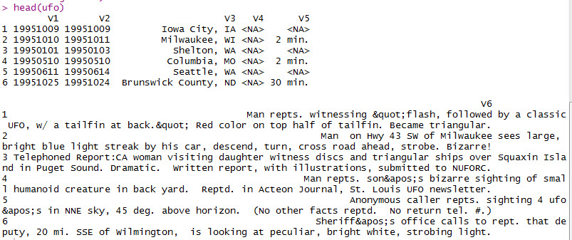
#names()既可以写入列名，也可以读取列名

names(ufo) <- c("DateOccurred", "DateReported", "Location", 
                "ShortDescription", "Duration", "LongDescription")

#as.Date用法，可以将字符串转为Date对象，具体格式可以设定，参考help

#错误：输入过长，考虑有畸形数据
#畸形数据处理

head(ufo[which(nchar(ufo$DateOccurred) != 8 
               | nchar(ufo$DateReported) != 8), 1])

#新建向量，布尔值F为不符合要求的行
#计数不符要求的行数，并只留下符合要求的行

good.rows <- ifelse(nchar(ufo$DateOccurred) != 8 
                    | nchar(ufo$DateReported) != 8, FALSE, TRUE)
length(which(!good.rows))
ufo <- ufo[good.rows, ]

　　运行结果是731条，而书上是371条，应该是书上有误

#转换

ufo$DateOccurred <- as.Date(ufo$DateOccurred, format = "%Y%m%d")
ufo$DateReported <- as.Date(ufo$DateReported, format = "%Y%m%d")

#输入为字符串，进行目击地点清洗
#strsplit用于分割字符串，在遇到不符条件的字符串会抛出异常，由tryCatch捕获，并返回缺失
#gsub将原始数据中的空格去掉（通过替换）
#条件语句用于检查是否多个逗号，返回缺失

get.location <- function(l){
  split.location <- tryCatch(strsplit(l, ",")[[1]], error = function(e) return(c(NA, NA)))
  clean.location <- gsub("^ ", "", split.location)
  if(length(clean.location) > 2){
    return(c(NA, NA))
  }
  else{
    return(clean.location)
  }
}

#lapply(list-apply)将function逐一用到向量元素上，并返回链表（list）

city.state <- lapply(ufo$Location, get.location)

#将list转换成matrix
#do.call在一个list上执行一个函数调用
#transform函数给ufo创建两个新列，tolower函数将大写变小写，为了统一格式

location.matrix <- do.call(rbind, city.state)
ufo <- transform(ufo, USCity = location.matrix[, 1], USState = tolower(location.matrix[, 2]), 
                 stringsAsFactors = FALSE)

#识别非美国地名，并置为NA

us.states <- c("ak", "al", "ar", "az", "ca", "co", "ct", "de", "fl", "ga", "hi", "ia", "id", 
               "il", "in", "ks", "ky", "la", "ma", "md", "me", "mi", "mn", "mo", "ms", "mt", 
               "nc", "nd", "ne", "nh", "nj", "nm", "nv", "ny", "oh", "ok", "or", "pa", "ri", 
               "sc", "sd", "tn", "tx", "ut", "va", "vt", "wa", "wi", "wv", "wy")
ufo$USState <- us.states[match(ufo$USState, us.states)]
ufo$USCity[is.na(ufo$USState)] <- NA

#只留下美国境内的记录

ufo.us <- subset(ufo, !is.na(USState))

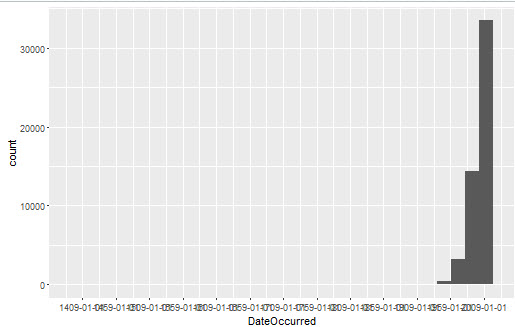
#对时间维度进行分析：
#预处理：对时间范围进行概述

summary(ufo.us$DateOccurred)
quick.hist <- ggplot(ufo.us, aes(x = DateOccurred)) + geom_histogram() + scale_x_date(date_breaks = "50 years")
print(quick.hist)

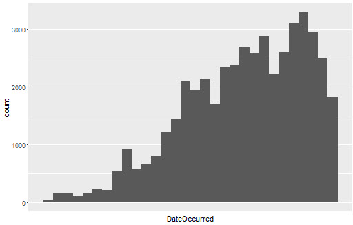
#取出1990年后的数据并作图

ufo.us <- subset(ufo.us, DateOccurred >= as.Date("1990-01-01"))
quick.hist.new <- ggplot(ufo.us, aes(x = DateOccurred)) + geom_histogram() + scale_x_date(date_breaks = "50 years")
print(quick.hist.new)

#统计每个年-月的目击个数
#时间信息转化为以月为单位，每个月的目击次数的数据框
#产生一个以月为单位的序列，包含了所有月信息，并与地点相结合生成数据框

ufo.us$YearMonth <- strftime(ufo.us$DateOccurred, format = "%Y-%m")
sightings.counts <- ddply(ufo.us, .(USState, YearMonth), nrow)
date.range <- seq.Date(from = as.Date(min(ufo.us$DateOccurred)), 
                       to = as.Date(max(ufo.us$DateOccurred)), by = "month")
date.strings <- strftime(date.range, "%Y-%m")
states.dates <- lapply(us.states, function(s) cbind(s, date.strings))
states.dates <- data.frame(do.call(rbind, states.dates), stringsAsFactors = FALSE)

#将两个数据框合并，merge函数，传入两个数据框，可以将相同的列合并，by.x和by.y指定列名
#all置为TRUE可以将未匹配处填充为NA
#进一步将all.sithtings细节优化，包括缺失值置0和转化变量类型

all.sightings <- merge(states.dates, sightings.counts, 
                       by.x = c("s", "date.strings"), 
                       by.y = c("USState", "YearMonth"), all = TRUE)
names(all.sightings) <- c("State", "YearMonth", "Sightings")
all.sightings$Sightings[is.na(all.sightings$Sightings)] <- 0
all.sightings$YearMonth <- as.Date(rep(date.range, length(us.states)))
all.sightings$State <- as.factor(toupper(all.sightings$State))

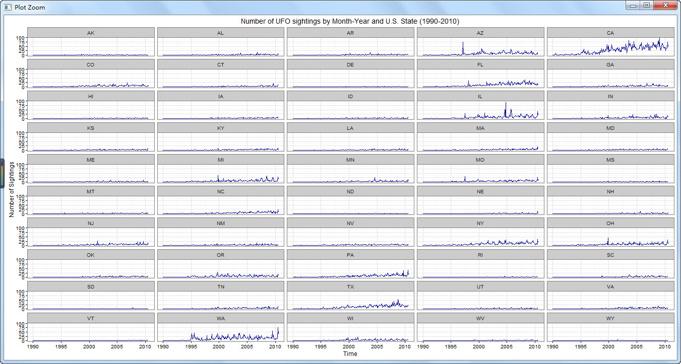
#分析数据
#geom_line表示曲线图，facet_wrap用于创建分块绘制的图形，并使用分类变量State
#theme_bw设定了图形背景主题
#scale_color_manual定义第二行中字符串"darkblue"的值，这个值相当于"darkblue"对应的值

state.plot <- ggplot(all.sightings, aes(x = YearMonth, y = Sightings)) + 
  geom_line(aes(color = "darkblue")) + 
  facet_wrap(~State, nrow = 10, ncol = 5) + 
  theme_bw() + 
  scale_color_manual(values = c("darkblue" = "darkblue"), guide = "none") + 
  xlab("Time") + 
  ylab("Number of Sightings") + 
  ggtitle("Number of UFO sightings by Month-Year and U.S. State (1990-2010)")
print(state.plot)