一、常量的定义
import tensorflow as tf
#类比  语法  api  原理
#基础数据类型  运算符  流程 字典 数组
data1 = tf.constant(2,dtype=tf.int32)
data2 = tf.Variable(10,name='var')
print(data1)
print(data2)
#shape 维度 const长度 shape维度 dtype 数据类型
sess = tf.Session()
print(sess.run(data1))
init = tf.global_variables_initializer()
sess.run(init)
print(sess.run(data2))
必须通过session来操作对象
二、tensorflow运行实质
tensorflow运算实质是由 tensor + 计算图
tensor 数据
op operation 赋值,运算
graphs 数据操作的过程
session 是执行的核心
import tensorflow as tf
#类比  语法  api  原理
#基础数据类型  运算符  流程 字典 数组
data1 = tf.constant(2,dtype=tf.int32)
data2 = tf.Variable(10,name='var')
print(data1)
print(data2)
#shape 维度 const长度 shape维度 dtype 数据类型
'''
sess = tf.Session()
print(sess.run(data1))
init = tf.global_variables_initializer()
sess.run(init)
print(sess.run(data2))
'''
init = tf.global_variables_initializer()
sess = tf.Session()
with sess:
    sess.run(init)
    print(sess.run(data2))
四则运算:
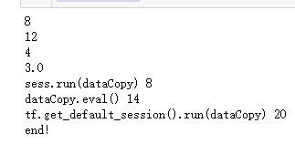
import tensorflow as tf
data1 = tf.constant(6)
data2 = tf.Variable(2)
dataAdd = tf.add(data1,data2)
dataCopy = tf.assign(data2,dataAdd)  #先把 6 和2进行计算
dataMul = tf.multiply(data1,data2)
dataSub = tf.subtract(data1,data2)
dataDiv = tf.divide(data1,data2)
init = tf.global_variables_initializer()
with tf.Session() as sess:
    sess.run(init)
    print(sess.run(dataAdd))
    print(sess.run(dataMul))
    print(sess.run(dataSub))
    print(sess.run(dataDiv))
    print('sess.run(dataCopy)',sess.run(dataCopy))
    print('dataCopy.eval()',dataCopy.eval())#eval的用法与下行一样
    print('tf.get_default_session().run(dataCopy)',tf.get_default_session().run(dataCopy))
print("end!")
运行结果:
3、矩阵
placehold 预定义变量
#placehold 预定义
import tensorflow as tf
data1 = tf.placeholder(tf.float32)
data2 = tf.placeholder(tf.float32)
dataAdd = tf.add(data1,data2)
with tf.session() as sess:
    print(sess.run(dataAdd,feed_dict=(data1:6,data2:2)))
    # 1 dataAdd 2 data (feed_dict = {1:6 2})
print('end')
基本操作
import tensorflow as tf
data1 = tf.constant([[6,6]])
data2 = tf.constant([[2],
                    [2]])
data3 = tf.constant([[3,3]])
data4 = tf.constant([[1,2],[3,4],[5,6]])
print(data4.shape)#打印维度
with tf.Session() as sess:
    print(sess.run(data4))#打印整体内容
    print(sess.run(data4[0]))#打印某一行
    print(sess.run(data4[:,1]))#打印某一列
    print(sess.run(data4[1,1]))#打印第一行第一列
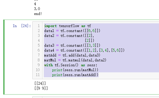
基本操作
import tensorflow as tf
data1 = tf.constant([[6,6]])
data2 = tf.constant([[2],
                    [2]])
data3 = tf.constant([[3,3]])
data4 = tf.constant([[1,2],[3,4],[5,6]])
matAdd = tf.add(data1,data3)
matMul = tf.matmul(data1,data2)
with tf.Session() as sess:
    print(sess.run(matMul))
    print(sess.run(matAdd))
import tensorflow as tf
mat0 = tf.constant([[0,0,0],[0,0,0]])
mat1 = tf.zeros([2,3])
mat2 = tf.ones([3,2])
mat3 = tf.fill([2,3],15)
with tf.Session() as sess:
    #print(sess.run(mat0))
    print(sess.run(mat1))
    print(sess.run(mat2))
    print(sess.run(mat3))
运行结果:

import tensorflow as tf
mat1 = tf.constant([[2],[3],[4]])
mat2 = tf.zeros_like(mat1)
mat3 = tf.linspace(0.0,2.0,11)
mat4 = tf.random_uniform([2,3],-1,2)
with tf.Session() as sess:
    print(sess.run(mat2))
    print(sess.run(mat3))
    print(sess.run(mat4))

四、Numpy的使用
#CRUD
import numpy as np
data1 = np.array([1,2,3,4,5])
print(data1)
data2 = np.array([[1,2],
                 [3,4]])
print(data2)
#维度
print(data1.shape,data2.shape)
#zero ones 单位矩阵
print(np.zeros([2,3]),np.ones([2,2]))
#改查
data2[1,0] = 5
print(data2)
print(data2[1,1])
#加减乘除
data3 = np.ones([2,3])
print(data3*2)
print(data3/3)
print(data3+2)
print(data3-3)
#矩阵的加法和乘法
data4 = np.array([[1,2,3],[4,5,6]])
print(data3+data4)
#
五、matplotlib的使用
绘制折线图
import numpy as np
import matplotlib.pyplot as plt
x = np.array([1,2,3,4,5,6,7,8])
y = np.array([3,4,7,6,2,7,10,15])
plt.plot(x,y,'r')#绘制 1 折线图 1x 2 y 3 color

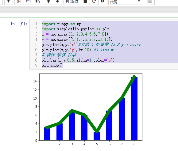
柱状图:
import numpy as np
import matplotlib.pyplot as plt
x = np.array([1,2,3,4,5,6,7,8])
y = np.array([3,4,7,6,2,7,10,15])
plt.plot(x,y,'r')#绘制 1 折线图 1x 2 y 3 color
plt.plot(x,y,'g',lw=10) #4 line w
# 折线 饼状 柱状
plt.bar(x,y,0.5,alpha=1,color='b')
plt.show()
神经网络逼近股票收盘价格
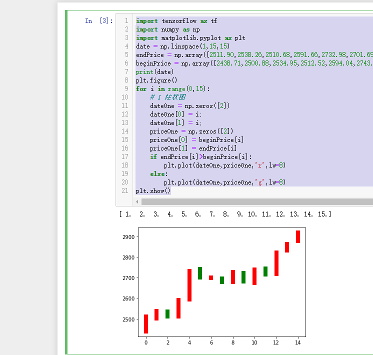
首先绘制K线
import tensorflow as tf
import numpy as np
import matplotlib.pyplot as plt
date = np.linspace(1,15,15)
endPrice = np.array([2511.90,2538.26,2510.68,2591.66,2732.98,2701.69,2701.29,2678.67,2726.50,2681.50,2739.17,2715.07,2823.58,2864.90,2919.08])
beginPrice = np.array([2438.71,2500.88,2534.95,2512.52,2594.04,2743.26,2697.47,2695.24,2678.23,2722.13,2674.93,2744.13,2717.46,2832.73,2877.40])
print(date)
plt.figure()
for i in range(0,15):
    # 1 柱状图
    dateOne = np.zeros([2])
    dateOne[0] = i;
    dateOne[1] = i;
    priceOne = np.zeros([2])
    priceOne[0] = beginPrice[i]
    priceOne[1] = endPrice[i]
    if endPrice[i]>beginPrice[i]:
        plt.plot(dateOne,priceOne,'r',lw=8)
    else:
        plt.plot(dateOne,priceOne,'g',lw=8)
plt.show()
实现人工神经网络:
分为三层:
1、输入层
2、中间层(隐藏层)
3、输出层
在这里面 输入矩阵为15 x 1
隐藏层矩阵 1x10的矩阵
输出层 输出矩阵
15 x 1
实现的功能:
通过天数输入 输出每天对应的股价
隐藏层
A*W1+b1 = B
B*w2+b2 = C
A:输入层 B:隐藏层 C:输出层 W1 1x10 B1 1x10偏移矩阵
代码如下:
# layer1:激励函数+乘加运算
import tensorflow as tf
import numpy as np
import matplotlib.pyplot as plt
date = np.linspace(1,15,15)
endPrice = np.array([2511.90,2538.26,2510.68,2591.66,2732.98,2701.69,2701.29,2678.67,2726.50,2681.50,2739.17,2715.07,2823.58,2864.90,2919.08]
)
beginPrice = np.array([2438.71,2500.88,2534.95,2512.52,2594.04,2743.26,2697.47,2695.24,2678.23,2722.13,2674.93,2744.13,2717.46,2832.73,2877.40])
print(date)
plt.figure()
for i in range(0,15):
    # 1 柱状图
    dateOne = np.zeros([2])
    dateOne[0] = i;
    dateOne[1] = i;
    priceOne = np.zeros([2])
    priceOne[0] = beginPrice[i]
    priceOne[1] = endPrice[i]
    if endPrice[i]>beginPrice[i]:
        plt.plot(dateOne,priceOne,'r',lw=8)
    else:
        plt.plot(dateOne,priceOne,'g',lw=8)
#plt.show()
# A(15x1)*w1(1x10)+b1(1*10) = B(15x10)
# B(15x10)*w2(10x1)+b2(15x1) = C(15x1)
# 1 A B C
dateNormal = np.zeros([15,1])
priceNormal = np.zeros([15,1])
for i in range(0,15):
    dateNormal[i,0] = i/14.0;
    priceNormal[i,0] = endPrice[i]/3000.0;
x = tf.placeholder(tf.float32,[None,1])
y = tf.placeholder(tf.float32,[None,1])
# B
w1 = tf.Variable(tf.random_uniform([1,10],0,1))
b1 = tf.Variable(tf.zeros([1,10]))
wb1 = tf.matmul(x,w1)+b1
layer1 = tf.nn.relu(wb1) # 激励函数
# C
w2 = tf.Variable(tf.random_uniform([10,1],0,1))
b2 = tf.Variable(tf.zeros([15,1]))
wb2 = tf.matmul(layer1,w2)+b2
layer2 = tf.nn.relu(wb2)
loss = tf.reduce_mean(tf.square(y-layer2))#y 真实 layer2 计算
train_step = tf.train.GradientDescentOptimizer(0.1).minimize(loss)
with tf.Session() as sess:
    sess.run(tf.global_variables_initializer())
    for i in range(0,10000):
        sess.run(train_step,feed_dict={x:dateNormal,y:priceNormal})
    # w1w2 b1b2  A + wb -->layer2
    pred = sess.run(layer2,feed_dict={x:dateNormal})
    predPrice = np.zeros([15,1])
    for i in range(0,15):
        predPrice[i,0]=(pred*3000)[i,0]
    plt.plot(date,predPrice,'b',lw=1)
plt.show()
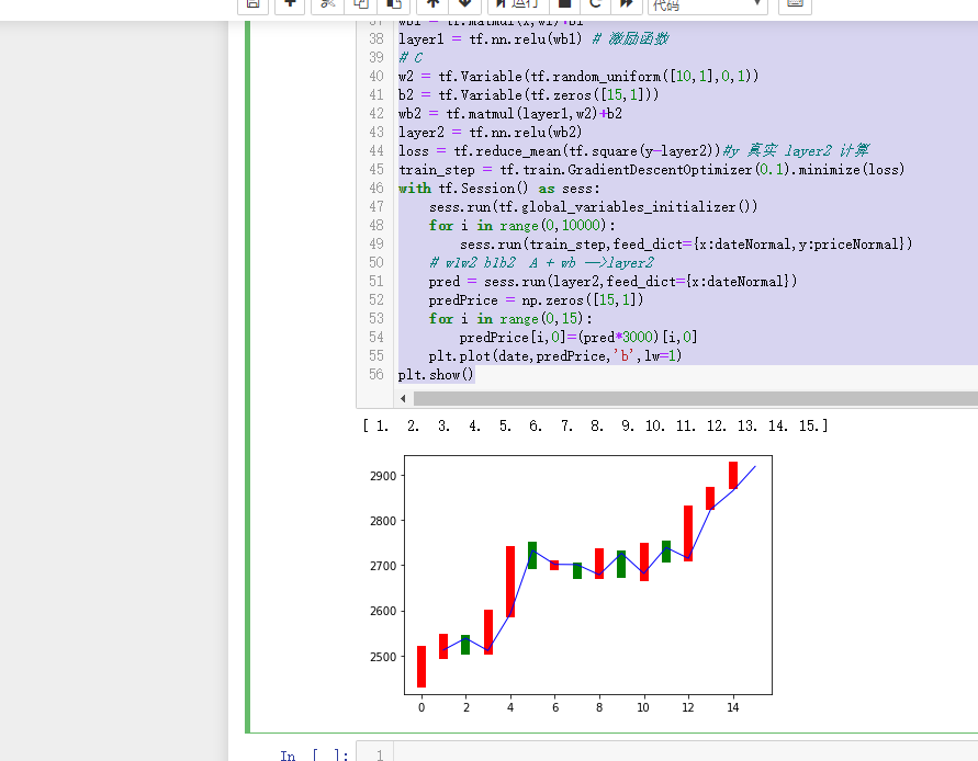
预计结果基本上吻合