处理序列化特征
wide and deep
线性模型+神经网络模型
Wide部分设置很有意思,作者为什么这么做呢?结合业务思考,在Google Play商店的app下载中,不断有新的app推出,并且有很多“非常冷门、小众”的app,而现在的智能手机user几乎全部会安装一系列必要的app。联想前面对Memorization和Generalization的介绍,此时的Deep部分无法很好的为这些app学到有效的embeddding,而这时Wide可以发挥了它“记忆”的优势,作者在这里选择了“记忆”user下载的app与被推荐的app之间的相关性,有点类似“装个这个app后还可能会装什么”。对于Wide来说,它现在的任务是弥补Deep的缺陷,其他大部分的活就交给Deep了,所以这时的Wide相比单独Wide也显得非常“轻量级”,这也是Join相对于Ensemble的优势。
记忆(memorization)即从历史数据中发现item或者特征之间的相关性。
泛化(generalization)即相关性的传递,发现在历史数据中很少或者没有出现的新的特征组合。
wide
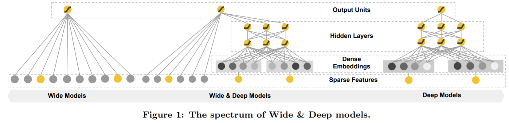
The wide component is a generalized linear model of the form (y=mathbf{w}^{T} mathbf{x}+b,) as illustrated in Figure 1 (left).(y) is the prediction,
(mathbf{x}=left[x_{1}, x_{2}, ldots, x_{d} ight]) is a vector of (d) features, (mathbf{w}=) (left[w_{1}, w_{2}, ldots, w_{d} ight]) are the model parameters and (b) is the bias.
wide 模型是广义的的线性模型
The feature set includes raw input features and transformed,One of the most important transformations is the cross-product transformation, which is defined as:
特征包括原始特征和转换特征,一个重要的转换特征是特征交叉项,
where (c_{k i}) is a boolean variable that is 1 if the (i) -th feature is part of the (k) -th transformation (phi_{k},) and 0 otherwise.
For binary features, a cross-product transformation (e.g., "AND(gender=female, language=en)") is 1 if and only if the constituent features ("gender=female" and "language=en") are all 1, and 0 otherwise. This captures the interactions between the binary features, and adds nonlinearity to the generalized linear model.
对于一个二分类的特征对于and,只有都满足条件的时候才为true,交叉项特征能过够给线性模型增加非线性。
我理解的交叉型特征其实就是做了一个特征融合,不过采用的计算方法是相乘
deep
The deep component is a feed-forward neural network, as shown in Figure 1 (right). For categorical features, the original inputs are feature strings (e.g., “language=en”). Each of these sparse, **high-dimensional categorical features are first converted into a low-dimensional and dense real-valued
vector, often referred to as an embedding vector. **The dimensionality of the embeddings are usually on the order of O(10) to O(100). The embedding vectors are initialized randomly and then the values are trained to minimize the final loss function during model training. These low-dimensional dense embedding vectors are then fed into the hidden layers of a neural network in the forward pass. Specifically, each hidden layer performs the following computation:
deep就是一个前馈神经网络
对于类别特征需要做一个embedding,将高维的类别特征转化为低维的dense层
从paper中选择了几张图
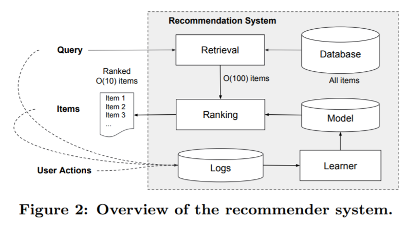
An overview of the app recommender system is shown in Figure 2. A query, which can include various user and contextual features, is generated when a user visits the app store. The recommender system returns a list of apps (also referred to as impressions) on which users can perform certain actions such as clicks or purchases. These user actions, along with the queries and impressions, are recorded in the logs as the training data for the learner.
系统的结构图图2所示。当用户访问商店的时候,包含用户和上下文信息的多种特征作为推荐系统的输入,推荐系统返回一个app列表。用户可能会点击或购买这些app。用户的这些行为会被记录,作为模型的训练数据。
wide & deep
The wide component and deep component are combined using a weighted sum of their output log odds as the pre-diction, which is then fed to one common logistic loss function for joint training. Note that there is a distinction between joint training and ensemble. In an ensemble, individual models are trained separately without knowing each other, and their predictions are combined only at inference time but not at training time. In contrast, joint training optimizes all parameters simultaneously by taking both the wide and deep part as well as the weights of their sum into account at training time. There are implications on model size too: For an ensemble, since the training is disjoint, each individual model size usually needs to be larger (e.g., with more features and transformations) to achieve reasonable accuracy for an ensemble to work. In comparison, for joint training the wide part only needs to complement the weaknesses of the deep part with a small number of cross-product feature transformations, rather than a full-size wide model.
wide & deep 做联合训练的时候和集成是不一样的
联合训练(joint training)有别于集成(ensemble),集成中训练阶段多个模型是独立分开训练的,并不知道彼此的存在,在预测阶段预测值综合了多个模型的预测值。相反,联合训练阶段则同时训练多个模型,共同优化参数。
集成模型独立训练,模型规模要大一些才能达到可接受的效果。而联合训练模型中,Wide部分只需补充Deep模型的缺点,即记忆能力,这部分主要通过小规模的交叉特征实现。因此联合训练模型的Wide部分的模型特征较小。
feature transformations, rather than a full-size wide model.
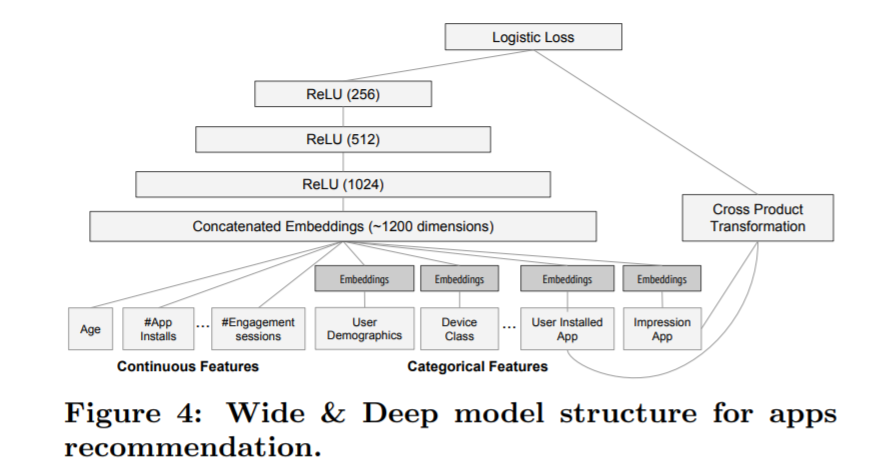
Joint training of a Wide & Deep Model is done by backpropagating the gradients from the output to both the wide and deep part of the model simultaneously using mini-batch stochastic optimization. In the experiments, we used Followthe-regularized-leader (FTRL) algorithm [3] with L1 regularization as the optimizer for the wide part of the model, and AdaGrad [1] for the deep part.The combined model is illustrated in Figure 1 (center).For a logistic regression problem, the model’s prediction is:
用FTRL算法优化wide部分的参数,AdaGrad算法优化深度部分的参数
(P(Y=1 | mathbf{x})=sigmaleft(mathbf{w}_{ ext {wide}}^{T}[mathbf{x}, phi(mathbf{x})]+mathbf{w}_{ ext {deep}}^{T} a^{left(l_{f} ight)}+b ight))
因此可以用这个框架做序列特征,学长给的这个demo理解起来确实很方便
不过里面deep的部分可优化的地方很多
前馈神经网络很多,可以结合transformer ,bert等进行结果
线性模型是通过交叉项来产出新的特征的,看似简单,也必不可少。
Memorization:
之前大规模稀疏输入的处理是:通过线性模型 + 特征交叉。所带来的Memorization以及记忆能力非常有效和可解释。但是Generalization(泛化能力)需要更多的人工特征工程。
Generalization:
相比之下,DNN几乎不需要特征工程。通过对低纬度的dense embedding进行组合可以学习到更深层次的隐藏特征。但是,缺点是有点over-generalize(过度泛化)。推荐系统中表现为:会给用户推荐不是那么相关的物品,尤其是user-item矩阵比较稀疏并且是high-rank(高秩矩阵)
两者区别:
Memorization趋向于更加保守,推荐用户之前有过行为的items。相比之下,generalization更加趋向于提高推荐系统的多样性(diversity)。
Wide & Deep:
Wide & Deep包括两部分:线性模型 + DNN部分。结合上面两者的优点,平衡memorization和generalization。
原因:综合memorization和generalizatio的优点,服务于推荐系统。相比于wide-only和deep-only的模型,wide & deep提升显著(这么比较脸是不是有点大。。。)
轻春
FM和DNN都算是这样的模型,可以在很少的特征工程情况下,通过学习一个低纬度的embedding vector来学习训练集中从未见过的组合特征。
FM和DNN的缺点在于:当query-item矩阵是稀疏并且是high-rank的时候(比如user有特殊的爱好,或item比较小众),很难非常效率的学习出低维度的表示。这种情况下,大部分的query-item都没有什么关系。但是dense embedding会导致几乎所有的query-item预测值都是非0的,这就导致了推荐过度泛化,会推荐一些不那么相关的物品。
相反,linear model却可以通过cross-product transformation来记住这些exception rules,而且仅仅使用了非常少的参数。
总结一下:
线性模型无法学习到训练集中未出现的组合特征;
FM或DNN通过学习embedding vector虽然可以学习到训练集中未出现的组合特征,但是会过度泛化。
Wide & Deep Model通过组合这两部分,解决了这些问题。
wide部分用到的是用户的历史行为,就是比较靠谱
Wide Part
Wide Part其实是一个广义的线性模型
使用特征包括:
raw input 原始特征
cross-product transformation 组合特征
接下来我们用同一个例子来说明:你给model一个query(你想吃的美食),model返回给你一个美食,然后你购买/消费了这个推荐。 也就是说,推荐系统其实要学习的是这样一个条件概率: P(consumption | query, item)
Wide Part可以对一些特例进行memorization。比如AND(query=”fried chicken”, item=”chicken fried rice”)虽然从字符角度来看很接近,但是实际上完全不同的东西,那么Wide就可以记住这个组合是不好的,是一个特例,下次当你再点炸鸡的时候,就不会推荐给你鸡肉炒米饭了。
Deep Part
Deep Part通过学习一个低纬度的dense representation(也叫做embedding vector)对于每一个query和item,来泛化给你推荐一些字符上看起来不那么相关,但是你可能也是需要的。比如说:你想要炸鸡,Embedding Space中,炸鸡和汉堡很接近,所以也会给你推荐汉堡。
Embedding vectors被随机初始化,并根据最终的loss来反向训练更新。这些低维度的dense embedding vectors被作为第一个隐藏层的输入。隐藏层的激活函数通常使用ReLU。